54  Saving and Loading

This tutorial shows how to save and load objects in spotpython. It is split into the following parts:

• Section 54.3 shows how to save and load objects in spotpython, if spotpython is used as an optimizer.
• Section 54.4 shows how to save and load hyperparameter tuning experiments.
• Section 54.5 shows how to save and load PyTorch Lightning models.
• Section 54.6 shows how to convert a PyTorch Lightning model to a plain PyTorch model.

54.1 Required Python Packages

import os
import pprint
import numpy as np
from math import inf
import matplotlib.pyplot as plt
import torch
import torch.nn as nn
import torch.optim as optim
from torch.utils.data import DataLoader, TensorDataset
from torch.utils.data import random_split
from sklearn.datasets import load_diabetes
from sklearn.model_selection import train_test_split
from sklearn.preprocessing import StandardScaler

from spotpython.utils.file import (load_experiment, load_result, get_experiment_filename, load_and_run_spot_python_experiment)
from spotpython.spot import Spot
from spotpython.utils.init import (
    fun_control_init,
    design_control_init,
    surrogate_control_init,
    optimizer_control_init)
from spotpython.fun.objectivefunctions import Analytical
from spotpython.hyperparameters.values import get_tuned_hyperparameters
from spotpython.data.diabetes import Diabetes
from spotpython.hyperdict.light_hyper_dict import LightHyperDict
from spotpython.fun.hyperlight import HyperLight
from spotpython.utils.eda import print_exp_table
from spotpython.hyperparameters.values import set_hyperparameter, get_tuned_architecture
from spotpython.light.testmodel import test_model
from spotpython.light.loadmodel import load_light_from_checkpoint
from spotpython.utils.device import getDevice
from spotpython.utils.classes import get_removed_attributes_and_base_net
from spotpython.hyperparameters.optimizer import optimizer_handler

And we will suppress warnings in this notebook.

54.2 Quick Overview of spotpython Save and Load Functions

Because the most common use case is to save and load hyperparameter tuning experiments, the save_experiment and load_experiment functions are explained first. In the real- world setting, users specify an experiment on their local machine and then run the experiment on a remote machine. Then, the result file is copied back to the local machine and loaded for further analysis. So, the main steps can be summarized as follows:

1. Generate an experiment configuration on the local machine, say 42_exp.pkl. To generate the configuration, the fun_control dictionary has to be initialized with save_experiment=True.
2. Copy the configuration file to the remote machine.
3. Run the experiment on the remote machine. The run on the remote machine is started with the command load_and_run_spot_python_experiment(filename="42_exp.pkl"). This generates a result file, say 42_res.pkl.
4. Copy the result file back to the local machine. Analyze the results on the local machine as shown below.

As can be seen from these step, we will distinguish between experiment/design/configuration files (with _exp in the filename) and result files (with _res in the filename).

Example 54.1 (Save and Load Hyperparameter Tuning Experiment)  

1. Generate an experiment configuration on the local machine, say 42_exp.pkl as follows:

PREFIX = "42"
data_set = Diabetes()
fun_control = fun_control_init(
    save_experiment=True,
    PREFIX=PREFIX,
    fun_evals=inf,
    max_time=1,
    data_set = data_set,
    core_model_name="light.regression.NNLinearRegressor",
    hyperdict=LightHyperDict,
    _L_in=10,
    _L_out=1)

fun = HyperLight().fun

set_hyperparameter(fun_control, "optimizer", [ "Adadelta", "Adam", "Adamax"])
set_hyperparameter(fun_control, "l1", [3,4])
set_hyperparameter(fun_control, "epochs", [3,5])
set_hyperparameter(fun_control, "batch_size", [4,11])
set_hyperparameter(fun_control, "dropout_prob", [0.0, 0.025])
set_hyperparameter(fun_control, "patience", [2,3])

design_control = design_control_init(init_size=10)

print_exp_table(fun_control)

S = Spot(fun=fun,fun_control=fun_control, design_control=design_control)

module_name: light
submodule_name: regression
model_name: NNLinearRegressor
| name           | type   | default   |   lower |   upper | transform             |
|----------------|--------|-----------|---------|---------|-----------------------|
| l1             | int    | 3         |     3   |   4     | transform_power_2_int |
| epochs         | int    | 4         |     3   |   5     | transform_power_2_int |
| batch_size     | int    | 4         |     4   |  11     | transform_power_2_int |
| act_fn         | factor | ReLU      |     0   |   5     | None                  |
| optimizer      | factor | SGD       |     0   |   2     | None                  |
| dropout_prob   | float  | 0.01      |     0   |   0.025 | None                  |
| lr_mult        | float  | 1.0       |     0.1 |  10     | None                  |
| patience       | int    | 2         |     2   |   3     | transform_power_2_int |
| batch_norm     | factor | 0         |     0   |   1     | None                  |
| initialization | factor | Default   |     0   |   4     | None                  |
Experiment saved to 42_exp.pkl

As the output shows, the configuration is saved as a pickle-file that contains the full information. In our example, the filename is 42_exp.pkl.

2. Copy the configuration file to the remote machine. This can be done with the scp command, see below, but is omitted here for brevity.

3. Run the experiment on the remote machine. This step is simulated on the local machine for demonstration purposes. This generates a result file, say 42_res.pkl. This can be done with the following code:

# S_res = S.run() is NOT used here, because we want to simulate the remote run
# Instead, we use the load_and_run_spot_python_experiment function:
S_remote = load_and_run_spot_python_experiment(filename="42_exp.pkl")

Loaded experiment from 42_exp.pkl

train_model result: {'val_loss': 23075.09765625, 'hp_metric': 23075.09765625}

train_model result: {'val_loss': 3850.81201171875, 'hp_metric': 3850.81201171875}

train_model result: {'val_loss': 6251.13916015625, 'hp_metric': 6251.13916015625}

train_model result: {'val_loss': 24093.25390625, 'hp_metric': 24093.25390625}

train_model result: {'val_loss': 23622.310546875, 'hp_metric': 23622.310546875}

train_model result: {'val_loss': 3700.772216796875, 'hp_metric': 3700.772216796875}

train_model result: {'val_loss': 20202.96875, 'hp_metric': 20202.96875}

train_model result: {'val_loss': 14793.4892578125, 'hp_metric': 14793.4892578125}

train_model result: {'val_loss': 21675.736328125, 'hp_metric': 21675.736328125}

train_model result: {'val_loss': 23792.47265625, 'hp_metric': 23792.47265625}
train_model result: {'val_loss': 21009.76953125, 'hp_metric': 21009.76953125}
spotpython tuning: 3700.772216796875 [----------] 1.13% 

train_model result: {'val_loss': 4301.27197265625, 'hp_metric': 4301.27197265625}
spotpython tuning: 3700.772216796875 [----------] 3.10% 

train_model result: {'val_loss': 23374.458984375, 'hp_metric': 23374.458984375}
spotpython tuning: 3700.772216796875 [#---------] 6.60% 

train_model result: {'val_loss': 21645.3046875, 'hp_metric': 21645.3046875}
spotpython tuning: 3700.772216796875 [#---------] 8.36% 

train_model result: {'val_loss': 22940.349609375, 'hp_metric': 22940.349609375}
spotpython tuning: 3700.772216796875 [#---------] 9.67% 

train_model result: {'val_loss': 13541.41015625, 'hp_metric': 13541.41015625}
spotpython tuning: 3700.772216796875 [#---------] 11.28% 

train_model result: {'val_loss': 23418.01953125, 'hp_metric': 23418.01953125}
spotpython tuning: 3700.772216796875 [#---------] 13.08% 

train_model result: {'val_loss': 12708.07421875, 'hp_metric': 12708.07421875}
spotpython tuning: 3700.772216796875 [##--------] 18.50% 

train_model result: {'val_loss': 22581.041015625, 'hp_metric': 22581.041015625}
spotpython tuning: 3700.772216796875 [##--------] 19.95% 

train_model result: {'val_loss': 24149.140625, 'hp_metric': 24149.140625}
spotpython tuning: 3700.772216796875 [##--------] 21.73% 

train_model result: {'val_loss': 19953.34375, 'hp_metric': 19953.34375}
spotpython tuning: 3700.772216796875 [##--------] 24.27% 

train_model result: {'val_loss': 23658.99609375, 'hp_metric': 23658.99609375}
spotpython tuning: 3700.772216796875 [###-------] 25.34% 

train_model result: {'val_loss': 23863.802734375, 'hp_metric': 23863.802734375}
spotpython tuning: 3700.772216796875 [###-------] 30.31% 

train_model result: {'val_loss': 21391.634765625, 'hp_metric': 21391.634765625}
spotpython tuning: 3700.772216796875 [###-------] 31.34% 

train_model result: {'val_loss': 3141.2373046875, 'hp_metric': 3141.2373046875}
spotpython tuning: 3141.2373046875 [###-------] 32.98% 

train_model result: {'val_loss': 23955.75390625, 'hp_metric': 23955.75390625}
spotpython tuning: 3141.2373046875 [###-------] 34.04% 

train_model result: {'val_loss': 24121.322265625, 'hp_metric': 24121.322265625}
spotpython tuning: 3141.2373046875 [####------] 35.17% 

train_model result: {'val_loss': 23839.5078125, 'hp_metric': 23839.5078125}
spotpython tuning: 3141.2373046875 [####------] 36.80% 

train_model result: {'val_loss': 23634.453125, 'hp_metric': 23634.453125}
spotpython tuning: 3141.2373046875 [####------] 39.35% 

train_model result: {'val_loss': 21901.3046875, 'hp_metric': 21901.3046875}
spotpython tuning: 3141.2373046875 [####------] 41.26% 

train_model result: {'val_loss': 3335.79296875, 'hp_metric': 3335.79296875}
spotpython tuning: 3141.2373046875 [####------] 43.60% 

train_model result: {'val_loss': 23936.423828125, 'hp_metric': 23936.423828125}
spotpython tuning: 3141.2373046875 [#####-----] 45.27% 

train_model result: {'val_loss': 24018.939453125, 'hp_metric': 24018.939453125}
spotpython tuning: 3141.2373046875 [#####-----] 46.48% 

train_model result: {'val_loss': 18822.509765625, 'hp_metric': 18822.509765625}
spotpython tuning: 3141.2373046875 [#####-----] 47.79% 

train_model result: {'val_loss': nan, 'hp_metric': nan}

train_model result: {'val_loss': 23965.283203125, 'hp_metric': 23965.283203125}
spotpython tuning: 3141.2373046875 [#####-----] 49.65% 

train_model result: {'val_loss': 21826.103515625, 'hp_metric': 21826.103515625}
spotpython tuning: 3141.2373046875 [#####-----] 51.74% 

train_model result: {'val_loss': 24177.47265625, 'hp_metric': 24177.47265625}
spotpython tuning: 3141.2373046875 [#####-----] 52.67% 

train_model result: {'val_loss': nan, 'hp_metric': nan}

train_model result: {'val_loss': 11319.5859375, 'hp_metric': 11319.5859375}
spotpython tuning: 3141.2373046875 [#####-----] 54.61% 

train_model result: {'val_loss': 19436.45703125, 'hp_metric': 19436.45703125}
spotpython tuning: 3141.2373046875 [######----] 55.93% 

train_model result: {'val_loss': 16127.77734375, 'hp_metric': 16127.77734375}
spotpython tuning: 3141.2373046875 [######----] 59.01% 

train_model result: {'val_loss': 15944.9482421875, 'hp_metric': 15944.9482421875}
spotpython tuning: 3141.2373046875 [######----] 60.13% 

train_model result: {'val_loss': 3135.868408203125, 'hp_metric': 3135.868408203125}
spotpython tuning: 3135.868408203125 [#######---] 65.95% 

train_model result: {'val_loss': nan, 'hp_metric': nan}

train_model result: {'val_loss': 23784.703125, 'hp_metric': 23784.703125}
spotpython tuning: 3135.868408203125 [#######---] 67.34% 

train_model result: {'val_loss': 23250.484375, 'hp_metric': 23250.484375}
spotpython tuning: 3135.868408203125 [#######---] 69.44% 

train_model result: {'val_loss': 3622.6240234375, 'hp_metric': 3622.6240234375}
spotpython tuning: 3135.868408203125 [#######---] 74.46% 

train_model result: {'val_loss': 3191.072509765625, 'hp_metric': 3191.072509765625}
spotpython tuning: 3135.868408203125 [########--] 81.60% 

train_model result: {'val_loss': 3069.384521484375, 'hp_metric': 3069.384521484375}
spotpython tuning: 3069.384521484375 [#########-] 86.35% 

train_model result: {'val_loss': 3342.41064453125, 'hp_metric': 3342.41064453125}
spotpython tuning: 3069.384521484375 [#########-] 91.83% 

train_model result: {'val_loss': 3300.236083984375, 'hp_metric': 3300.236083984375}
spotpython tuning: 3069.384521484375 [##########] 97.18% 

train_model result: {'val_loss': 24049.640625, 'hp_metric': 24049.640625}
spotpython tuning: 3069.384521484375 [##########] 98.56% 

train_model result: {'val_loss': 3211.052001953125, 'hp_metric': 3211.052001953125}
spotpython tuning: 3069.384521484375 [##########] 100.00% Done...

Experiment saved to 42_res.pkl

A result file with the name 42_res.pkl is stored in the current directory.

4. Copy the result file back to the local machine. This can be done with the scp command, see below, but is omitted here for brevity. The result file can be loaded with the following code:

S_res = load_result(PREFIX="42")

Loaded experiment from 42_res.pkl

S_res.plot_progress(log_y=True)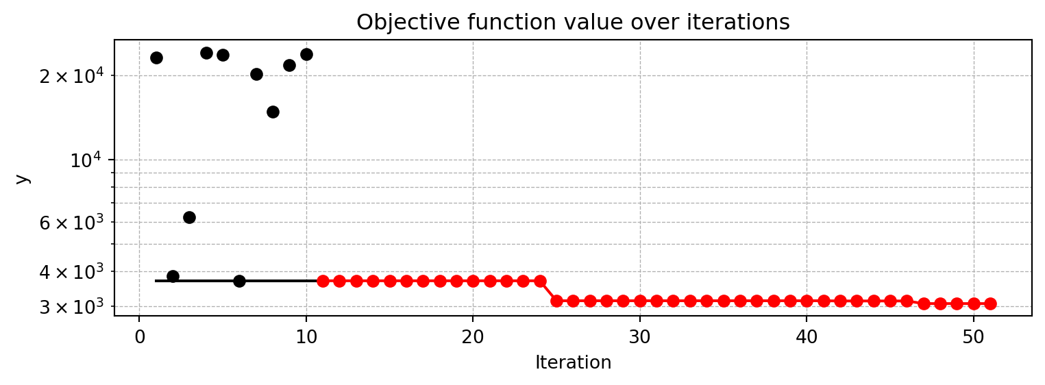

S_res.print_results()

min y: 3069.384521484375
l1: 3.0
epochs: 5.0
batch_size: 5.0
act_fn: 2.0
optimizer: 0.0
dropout_prob: 0.025
lr_mult: 10.0
patience: 3.0
batch_norm: 1.0
initialization: 3.0

[['l1', np.float64(3.0)],
 ['epochs', np.float64(5.0)],
 ['batch_size', np.float64(5.0)],
 ['act_fn', np.float64(2.0)],
 ['optimizer', np.float64(0.0)],
 ['dropout_prob', np.float64(0.025)],
 ['lr_mult', np.float64(10.0)],
 ['patience', np.float64(3.0)],
 ['batch_norm', np.float64(1.0)],
 ['initialization', np.float64(3.0)]]

If you add fun_control=S_res.fun_control as an argument to the get_tuned_hyperparameters function, the names of the hyperparameters are used as keys in the dictionary.

get_tuned_hyperparameters(S_res, fun_control=S_res.fun_control)

{'l1': np.float64(3.0),
 'epochs': np.float64(5.0),
 'batch_size': np.float64(5.0),
 'act_fn': 'ReLU',
 'optimizer': 'Adadelta',
 'dropout_prob': np.float64(0.025),
 'lr_mult': np.float64(10.0),
 'patience': np.float64(3.0),
 'batch_norm': 1,
 'initialization': 'xavier_uniform'}

Get the transformed hyperparameters that can be passed to the model.

config = get_tuned_architecture(S_res)
pprint.pprint(config)

{'act_fn': ReLU(),
 'batch_norm': True,
 'batch_size': 32,
 'dropout_prob': 0.025,
 'epochs': 32,
 'initialization': 'xavier_uniform',
 'l1': 8,
 'lr_mult': 10.0,
 'optimizer': 'Adadelta',
 'patience': 8}

After getting the tuned architecture, the model can be created and tested with the following code.

test_model(config, S_res.fun_control)

┏━━━━━━━━━━━━━━━━━━━━━━━━━━━┳━━━━━━━━━━━━━━━━━━━━━━━━━━━┓
┃        Test metric        ┃       DataLoader 0        ┃
┡━━━━━━━━━━━━━━━━━━━━━━━━━━━╇━━━━━━━━━━━━━━━━━━━━━━━━━━━┩
│         hp_metric         │     2675.995849609375     │
│         val_loss          │     2675.995849609375     │
└───────────────────────────┴───────────────────────────┘

test_model result: {'val_loss': 2675.995849609375, 'hp_metric': 2675.995849609375}

(2675.995849609375, 2675.995849609375)

S_res.plot_important_hyperparameter_contour(max_imp=3)

l1:  0.10828653263861841
epochs:  0.10828653263861841
batch_size:  25.46084190866584
act_fn:  0.10828653263861841
optimizer:  28.540816907178773
dropout_prob:  0.10828653263861841
lr_mult:  0.3258742416726233
patience:  0.5936371336313039
batch_norm:  100.0
initialization:  22.142487269666166

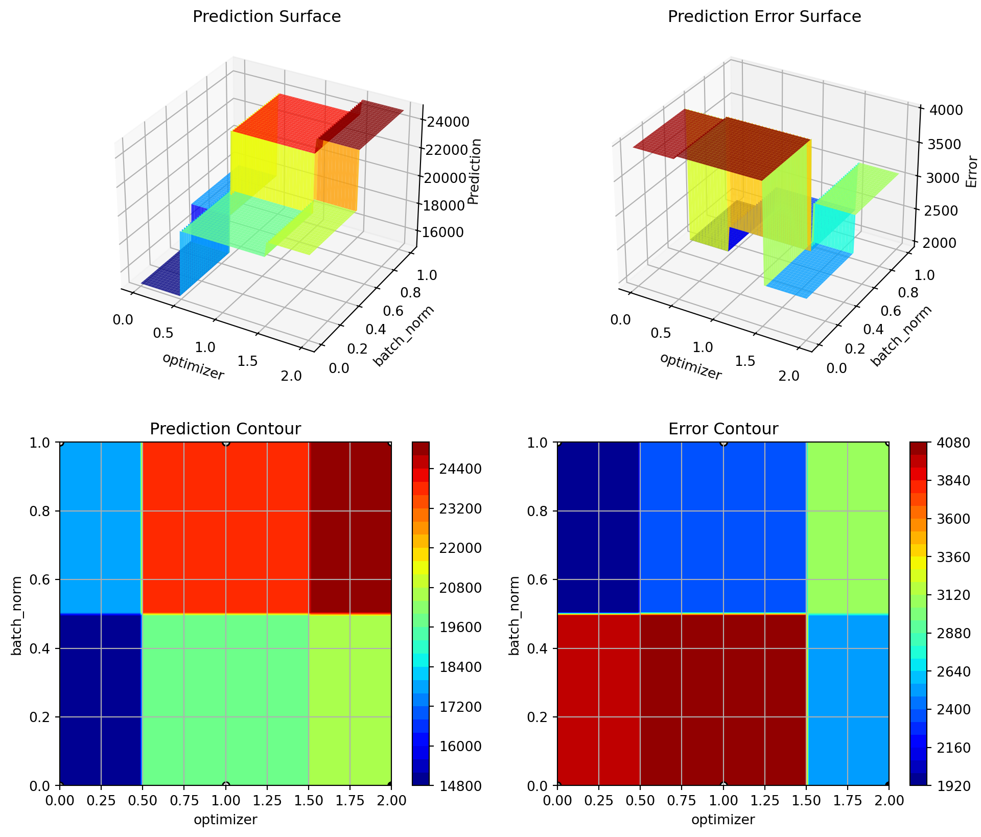
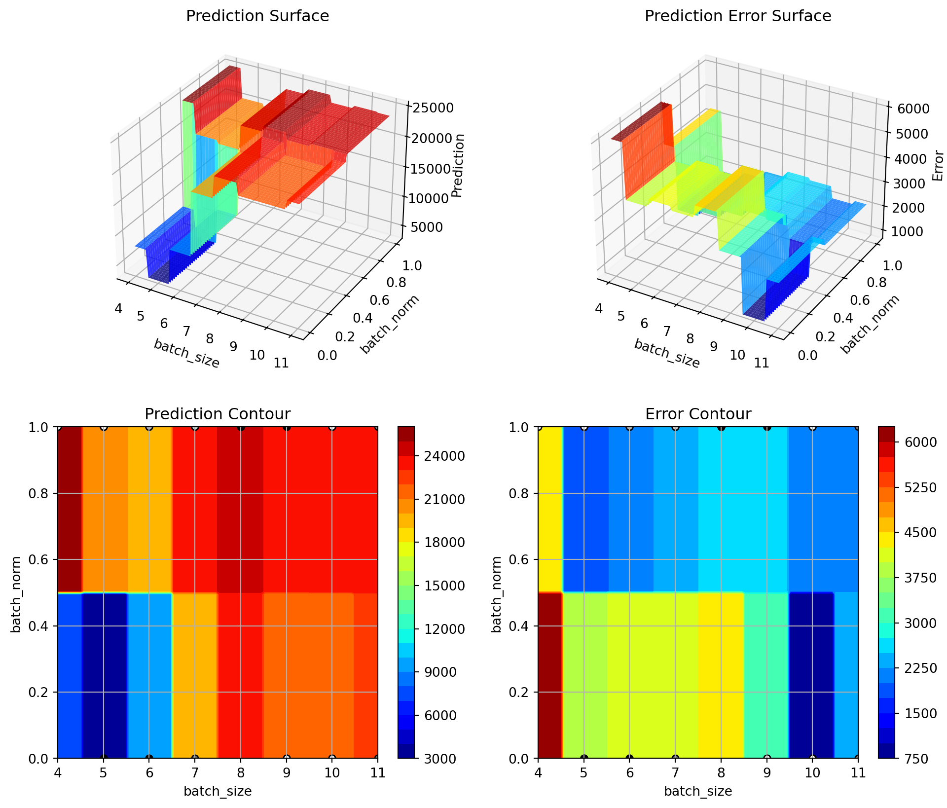
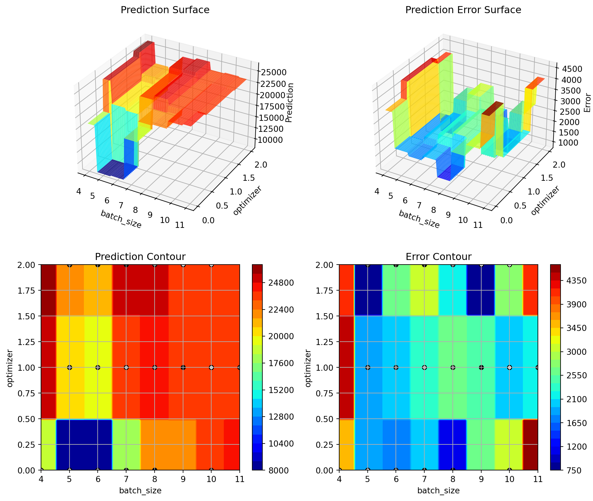
S_res.plot_importance()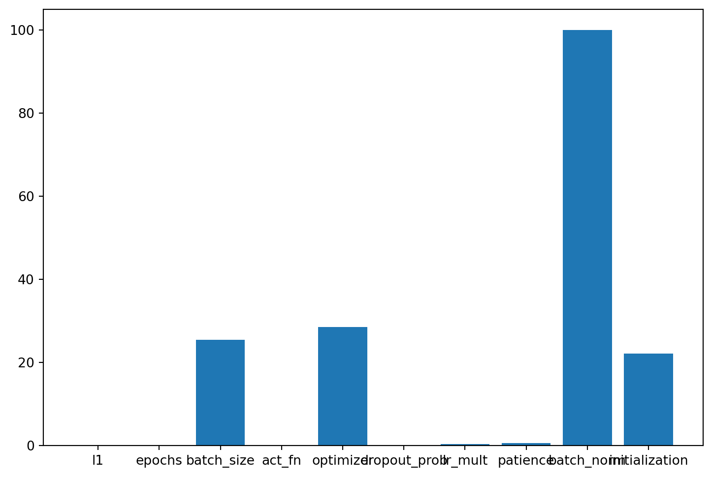

54.3 spotpython: Saving and Loading Optimization Experiments

In this section, we will show how results from spotpython can be saved and reloaded. Here, spotpython can be used as an optimizer. If spotpython is used as an optimizer, no dictionary of hyperparameters has be specified. The fun_control dictionary is sufficient.

PREFIX="branin"

fun = Analytical().fun_branin
fun_control = fun_control_init(
            PREFIX=PREFIX,
            lower = np.array([0, 0]),
            upper = np.array([10, 10]),
            fun_evals=8,
            fun_repeats=1,
            max_time=inf,
            noise=False,
            tolerance_x=0,
            ocba_delta=0,
            var_type=["num", "num"],
            infill_criterion="ei",
            n_points=1,
            seed=123,
            log_level=20,
            show_models=False,
            save_experiment=True,
            show_progress=True)
design_control = design_control_init(
            init_size=5,
            repeats=1)
surrogate_control = surrogate_control_init(
            model_fun_evals=10000,
            min_theta=-3,
            max_theta=3,
            theta_init_zero=True,
            n_p=1,
            optim_p=False,
            var_type=["num", "num"],
            seed=124)
optimizer_control = optimizer_control_init(
            max_iter=1000,
            seed=125)
S = Spot(fun=fun,
            fun_control=fun_control,
            design_control=design_control,
            surrogate_control=surrogate_control,
            optimizer_control=optimizer_control)
S.run()

Experiment saved to branin_exp.pkl
spotpython tuning: 4.7932399644479124 [########--] 75.00% 
spotpython tuning: 4.7932399644479124 [#########-] 87.50% 
spotpython tuning: 1.9923343958368207 [##########] 100.00% Done...

Experiment saved to branin_res.pkl

<spotpython.spot.spot.Spot at 0x354ffc620>

S_exp = load_experiment(PREFIX=PREFIX)

Loaded experiment from branin_exp.pkl

S_res = load_result(PREFIX=PREFIX)

Loaded experiment from branin_res.pkl

The progress of the original experiment is shown in Figure 54.1 and the reloaded experiment in Figure 54.2.

S.plot_progress(log_y=True)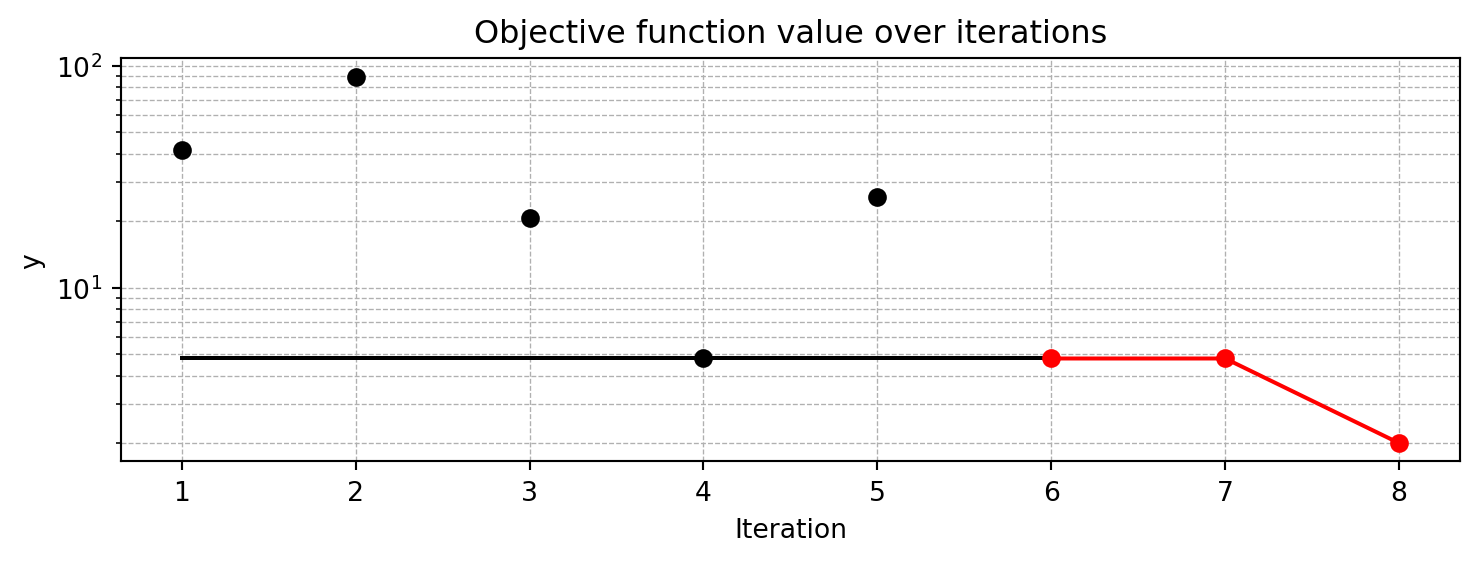

Figure 54.1: Progress of the original experiment

S_res.plot_progress(log_y=True)

Figure 54.2: Progress of the reloaded experiment

The results from the original experiment are shown in Table 54.1 and the reloaded experiment in Table 54.2.

S.print_results()

min y: 1.9923343958368207
x0: 3.7257814978658934
x1: 1.9085591905504409

Table 54.1

[['x0', np.float64(3.7257814978658934)],
 ['x1', np.float64(1.9085591905504409)]]

S_res.print_results()

min y: 1.9923343958368207
x0: 3.7257814978658934
x1: 1.9085591905504409

Table 54.2

[['x0', np.float64(3.7257814978658934)],
 ['x1', np.float64(1.9085591905504409)]]

54.3.1 Getting the Tuned Hyperparameters

The tuned hyperparameters can be obtained as a dictionary with the following code. Since spotpython is used as an optimizer, the numerical levels of the hyperparameters are identical to the optimized values of the underlying optimization problem, here: the Branin function.

get_tuned_hyperparameters(spot_tuner=S_res)

{'x0': np.float64(3.7257814978658934), 'x1': np.float64(1.9085591905504409)}

NoteSummary: Saving and Loading Optimization Experiments

• If spotpython is used as an optimizer (without an hyperparameter dictionary), experiments can be saved and reloaded with the save_experiment and load_experiment functions.
• The tuned hyperparameters can be obtained with the get_tuned_hyperparameters function.

54.4 spotpython as a Hyperparameter Tuner

If spotpython is used as a hyperparameter tuner, in addition to the fun_control dictionary a core_model dictionary has to be specified. Furthermore, a data set has to be selected and added to the fun_control dictionary. Here, we will use the Diabetes data set.

54.4.1 The Diabetes Data Set

The hyperparameter tuning of a PyTorch Lightning network on the Diabetes data set is used as an example. The Diabetes data set is a PyTorch Dataset for regression, which originates from the scikit-learn package, see https://scikit-learn.org/stable/modules/generated/sklearn.datasets.load_diabetes.html#sklearn.datasets.load_diabetes.

Ten baseline variables, age, sex, body mass index, average blood pressure, and six blood serum measurements were obtained for each of n = 442 diabetes patients, as well as the response of interest, a quantitative measure of disease progression one year after baseline. The Diabetes data set is has the following properties:

• Samples total: 442
• Dimensionality: 10
• Features: real, \(-.2 < x < .2\)
• Targets: integer \(25 - 346\)

data_set = Diabetes()

PREFIX="604"
fun_control = fun_control_init(
    save_experiment=True,
    PREFIX=PREFIX,
    fun_evals=inf,
    max_time=1,
    data_set = data_set,
    core_model_name="light.regression.NNLinearRegressor",
    hyperdict=LightHyperDict,
    _L_in=10,
    _L_out=1)

fun = HyperLight().fun

set_hyperparameter(fun_control, "optimizer", [ "Adadelta", "Adam", "Adamax"])
set_hyperparameter(fun_control, "l1", [3,4])
set_hyperparameter(fun_control, "epochs", [3,5])
set_hyperparameter(fun_control, "batch_size", [4,11])
set_hyperparameter(fun_control, "dropout_prob", [0.0, 0.025])
set_hyperparameter(fun_control, "patience", [2,3])

design_control = design_control_init(init_size=10)

print_exp_table(fun_control)

module_name: light
submodule_name: regression
model_name: NNLinearRegressor
| name           | type   | default   |   lower |   upper | transform             |
|----------------|--------|-----------|---------|---------|-----------------------|
| l1             | int    | 3         |     3   |   4     | transform_power_2_int |
| epochs         | int    | 4         |     3   |   5     | transform_power_2_int |
| batch_size     | int    | 4         |     4   |  11     | transform_power_2_int |
| act_fn         | factor | ReLU      |     0   |   5     | None                  |
| optimizer      | factor | SGD       |     0   |   2     | None                  |
| dropout_prob   | float  | 0.01      |     0   |   0.025 | None                  |
| lr_mult        | float  | 1.0       |     0.1 |  10     | None                  |
| patience       | int    | 2         |     2   |   3     | transform_power_2_int |
| batch_norm     | factor | 0         |     0   |   1     | None                  |
| initialization | factor | Default   |     0   |   4     | None                  |

In contrast to the default setting, where save_experiment is set to False, here the fun_control dictionary is initialized save_experiment=True. Alternatively, an existing fun_control dictionary can be updated with {"save_experiment": True} as shown in the following code.

fun_control.update({"save_experiment": True})

If save_experiment is set to True, the results of the hyperparameter tuning experiment are stored in a pickle file with the name PREFIX after the tuning is finished in the current directory.

Alternatively, the spot object and the corresponding dictionaries can be saved with the save_experiment method, which is part of the spot object. Therefore, the spot object has to be created as shown in the following code.

S_diabetes = Spot(fun=fun,fun_control=fun_control, design_control=design_control)
S_diabetes.save_experiment(path="userExperiment", overwrite=False)

Experiment saved to 604_exp.pkl
Error: File userExperiment/604_exp.pkl already exists. Use overwrite=True to overwrite the file.

Here, we have added a path argument to specify the directory where the experiment is saved. The resulting pickle file can be copied to another directory or computer and reloaded with the load_experiment function. It can also be used for performing the tuning run. Here, we will execute the tuning run on the local machine, which can be done with the following code.

S_diabetes_res = S_diabetes.run()

train_model result: {'val_loss': 23075.09765625, 'hp_metric': 23075.09765625}

train_model result: {'val_loss': 3850.81201171875, 'hp_metric': 3850.81201171875}

train_model result: {'val_loss': 6251.13916015625, 'hp_metric': 6251.13916015625}

train_model result: {'val_loss': 24093.25390625, 'hp_metric': 24093.25390625}

train_model result: {'val_loss': 23622.310546875, 'hp_metric': 23622.310546875}

train_model result: {'val_loss': 3700.772216796875, 'hp_metric': 3700.772216796875}

train_model result: {'val_loss': 20202.96875, 'hp_metric': 20202.96875}

train_model result: {'val_loss': 14793.4892578125, 'hp_metric': 14793.4892578125}

train_model result: {'val_loss': 21675.736328125, 'hp_metric': 21675.736328125}

train_model result: {'val_loss': 23792.47265625, 'hp_metric': 23792.47265625}
train_model result: {'val_loss': 21009.76953125, 'hp_metric': 21009.76953125}
spotpython tuning: 3700.772216796875 [----------] 1.12% 

train_model result: {'val_loss': 4301.27197265625, 'hp_metric': 4301.27197265625}
spotpython tuning: 3700.772216796875 [----------] 3.11% 

train_model result: {'val_loss': 23374.458984375, 'hp_metric': 23374.458984375}
spotpython tuning: 3700.772216796875 [#---------] 6.65% 

train_model result: {'val_loss': 21645.3046875, 'hp_metric': 21645.3046875}
spotpython tuning: 3700.772216796875 [#---------] 8.35% 

train_model result: {'val_loss': 22940.349609375, 'hp_metric': 22940.349609375}
spotpython tuning: 3700.772216796875 [#---------] 9.62% 

train_model result: {'val_loss': 13541.41015625, 'hp_metric': 13541.41015625}
spotpython tuning: 3700.772216796875 [#---------] 11.22% 

train_model result: {'val_loss': 23418.01953125, 'hp_metric': 23418.01953125}
spotpython tuning: 3700.772216796875 [#---------] 12.86% 

train_model result: {'val_loss': 12708.07421875, 'hp_metric': 12708.07421875}
spotpython tuning: 3700.772216796875 [##--------] 18.26% 

train_model result: {'val_loss': 22581.041015625, 'hp_metric': 22581.041015625}
spotpython tuning: 3700.772216796875 [##--------] 19.71% 

train_model result: {'val_loss': 24149.140625, 'hp_metric': 24149.140625}
spotpython tuning: 3700.772216796875 [##--------] 21.49% 

train_model result: {'val_loss': 19953.34375, 'hp_metric': 19953.34375}
spotpython tuning: 3700.772216796875 [##--------] 24.04% 

train_model result: {'val_loss': 23658.99609375, 'hp_metric': 23658.99609375}
spotpython tuning: 3700.772216796875 [###-------] 25.06% 

train_model result: {'val_loss': 23863.802734375, 'hp_metric': 23863.802734375}
spotpython tuning: 3700.772216796875 [###-------] 29.78% 

train_model result: {'val_loss': 21391.634765625, 'hp_metric': 21391.634765625}
spotpython tuning: 3700.772216796875 [###-------] 30.83% 

train_model result: {'val_loss': 3141.2373046875, 'hp_metric': 3141.2373046875}
spotpython tuning: 3141.2373046875 [###-------] 32.50% 

train_model result: {'val_loss': 23955.75390625, 'hp_metric': 23955.75390625}
spotpython tuning: 3141.2373046875 [###-------] 33.51% 

train_model result: {'val_loss': 24121.322265625, 'hp_metric': 24121.322265625}
spotpython tuning: 3141.2373046875 [###-------] 34.59% 

train_model result: {'val_loss': 23839.5078125, 'hp_metric': 23839.5078125}
spotpython tuning: 3141.2373046875 [####------] 36.05% 

train_model result: {'val_loss': 23634.453125, 'hp_metric': 23634.453125}
spotpython tuning: 3141.2373046875 [####------] 38.43% 

train_model result: {'val_loss': 21901.3046875, 'hp_metric': 21901.3046875}
spotpython tuning: 3141.2373046875 [####------] 40.31% 

train_model result: {'val_loss': 3335.79296875, 'hp_metric': 3335.79296875}
spotpython tuning: 3141.2373046875 [####------] 42.54% 

train_model result: {'val_loss': 23936.423828125, 'hp_metric': 23936.423828125}
spotpython tuning: 3141.2373046875 [####------] 44.20% 

train_model result: {'val_loss': 24018.939453125, 'hp_metric': 24018.939453125}
spotpython tuning: 3141.2373046875 [#####-----] 45.42% 

train_model result: {'val_loss': 18822.509765625, 'hp_metric': 18822.509765625}
spotpython tuning: 3141.2373046875 [#####-----] 46.73% 

train_model result: {'val_loss': nan, 'hp_metric': nan}

train_model result: {'val_loss': 23965.283203125, 'hp_metric': 23965.283203125}
spotpython tuning: 3141.2373046875 [#####-----] 48.58% 

train_model result: {'val_loss': 21826.103515625, 'hp_metric': 21826.103515625}
spotpython tuning: 3141.2373046875 [#####-----] 50.75% 

train_model result: {'val_loss': 24177.47265625, 'hp_metric': 24177.47265625}
spotpython tuning: 3141.2373046875 [#####-----] 51.64% 

train_model result: {'val_loss': nan, 'hp_metric': nan}

train_model result: {'val_loss': 11319.5859375, 'hp_metric': 11319.5859375}
spotpython tuning: 3141.2373046875 [#####-----] 53.64% 

train_model result: {'val_loss': 19436.45703125, 'hp_metric': 19436.45703125}
spotpython tuning: 3141.2373046875 [#####-----] 54.95% 

train_model result: {'val_loss': 16127.77734375, 'hp_metric': 16127.77734375}
spotpython tuning: 3141.2373046875 [######----] 58.02% 

train_model result: {'val_loss': 15944.9482421875, 'hp_metric': 15944.9482421875}
spotpython tuning: 3141.2373046875 [######----] 59.11% 

train_model result: {'val_loss': 3135.868408203125, 'hp_metric': 3135.868408203125}
spotpython tuning: 3135.868408203125 [######----] 64.84% 

train_model result: {'val_loss': nan, 'hp_metric': nan}

train_model result: {'val_loss': 23784.703125, 'hp_metric': 23784.703125}
spotpython tuning: 3135.868408203125 [#######---] 66.18% 

train_model result: {'val_loss': 23250.484375, 'hp_metric': 23250.484375}
spotpython tuning: 3135.868408203125 [#######---] 68.22% 

train_model result: {'val_loss': 3622.6240234375, 'hp_metric': 3622.6240234375}
spotpython tuning: 3135.868408203125 [#######---] 73.31% 

train_model result: {'val_loss': 3191.072509765625, 'hp_metric': 3191.072509765625}
spotpython tuning: 3135.868408203125 [########--] 80.39% 

train_model result: {'val_loss': 3069.384521484375, 'hp_metric': 3069.384521484375}
spotpython tuning: 3069.384521484375 [#########-] 85.14% 

train_model result: {'val_loss': 3342.41064453125, 'hp_metric': 3342.41064453125}
spotpython tuning: 3069.384521484375 [#########-] 90.60% 

train_model result: {'val_loss': 3300.236083984375, 'hp_metric': 3300.236083984375}
spotpython tuning: 3069.384521484375 [##########] 95.94% 

train_model result: {'val_loss': 24049.640625, 'hp_metric': 24049.640625}
spotpython tuning: 3069.384521484375 [##########] 97.33% 

train_model result: {'val_loss': 3211.052001953125, 'hp_metric': 3211.052001953125}
spotpython tuning: 3069.384521484375 [##########] 100.00% Done...

Experiment saved to 604_res.pkl

After the tuning run is finished, a pickle file with the name spot_604_experiment.pickle is stored in the local directory. This is a result of setting the save_experiment argument to True in the fun_control dictionary. We can load the experiment with the following code. Here, we have specified the PREFIX as an argument to the load_experiment function. Alternatively, the filename (filename) can be used as an argument.

S_diabetes_load_exp = load_experiment(PREFIX=PREFIX)
S_diabetes_load_res = load_result(PREFIX=PREFIX)

Loaded experiment from 604_exp.pkl
Loaded experiment from 604_res.pkl

For comparison, the tuned hyperparameters of the original experiment are shown first:

get_tuned_hyperparameters(S_diabetes, fun_control)

{'l1': np.float64(3.0),
 'epochs': np.float64(5.0),
 'batch_size': np.float64(5.0),
 'act_fn': 'ReLU',
 'optimizer': 'Adadelta',
 'dropout_prob': np.float64(0.025),
 'lr_mult': np.float64(10.0),
 'patience': np.float64(3.0),
 'batch_norm': 1,
 'initialization': 'xavier_uniform'}

Second, the tuned hyperparameters of the reloaded experiment are shown:

get_tuned_hyperparameters(S_diabetes_load_res)

{'l1': np.float64(3.0),
 'epochs': np.float64(5.0),
 'batch_size': np.float64(5.0),
 'act_fn': np.float64(2.0),
 'optimizer': np.float64(0.0),
 'dropout_prob': np.float64(0.025),
 'lr_mult': np.float64(10.0),
 'patience': np.float64(3.0),
 'batch_norm': np.float64(1.0),
 'initialization': np.float64(3.0)}

Note: The numerical levels of the hyperparameters are used as keys in the dictionary. If the fun_control dictionary is used, the names of the hyperparameters are used as keys in the dictionary.

get_tuned_hyperparameters(S_diabetes_load_res, fun_control=S_diabetes_load_exp.fun_control)

{'l1': np.float64(3.0),
 'epochs': np.float64(5.0),
 'batch_size': np.float64(5.0),
 'act_fn': 'ReLU',
 'optimizer': 'Adadelta',
 'dropout_prob': np.float64(0.025),
 'lr_mult': np.float64(10.0),
 'patience': np.float64(3.0),
 'batch_norm': 1,
 'initialization': 'xavier_uniform'}

Plot the progress of the original experiment are identical to the reloaded experiment.

S_diabetes.plot_progress()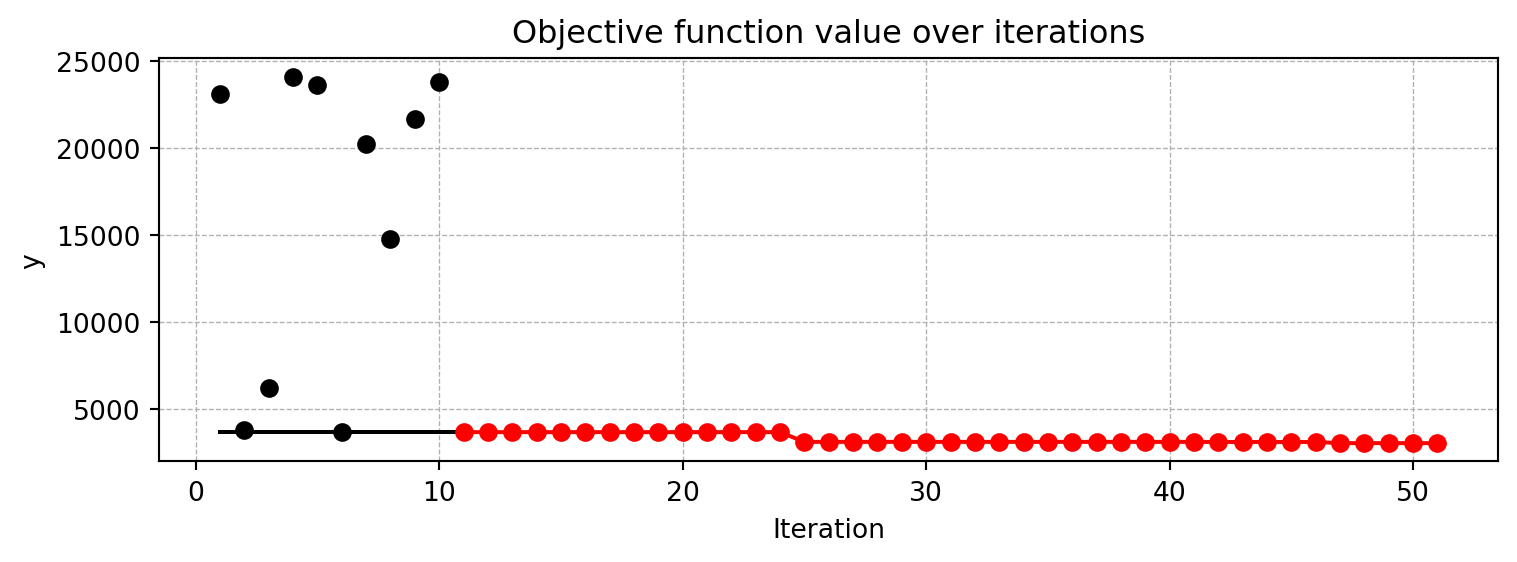

Figure 54.3

S_diabetes_load_res.plot_progress()

Figure 54.4

NoteSummary: Saving and Loading Hyperparameter-Tuning Experiments

• If spotpython is used as an hyperparameter tuner (with an hyperparameter dictionary), experiments can be saved and reloaded with the save_experiment and load_experiment functions.
• The tuned hyperparameters can be obtained with the get_tuned_hyperparameters function.

54.5 Saving and Loading PyTorch Lightning Models

Section 54.3 and Section 54.4 explained how to save and load optimization and hyperparameter tuning experiments and how to get the tuned hyperparameters as a dictionary. This section shows how to save and load PyTorch Lightning models.

54.5.1 Get the Tuned Architecture

In contrast to the function get_tuned_hyperparameters, the function get_tuned_architecture returns the tuned architecture of the model as a dictionary. Here, the transformations are already applied to the numerical levels of the hyperparameters and the encoding (and types) are the original types of the hyperparameters used by the model. Important: The config dictionary from get_tuned_architecture can be passed to the model without any modifications.

config = get_tuned_architecture(S_diabetes)
pprint.pprint(config)

{'act_fn': ReLU(),
 'batch_norm': True,
 'batch_size': 32,
 'dropout_prob': 0.025,
 'epochs': 32,
 'initialization': 'xavier_uniform',
 'l1': 8,
 'lr_mult': 10.0,
 'optimizer': 'Adadelta',
 'patience': 8}

After getting the tuned architecture, the model can be created and tested with the following code.

test_model(config, fun_control)

┏━━━━━━━━━━━━━━━━━━━━━━━━━━━┳━━━━━━━━━━━━━━━━━━━━━━━━━━━┓
┃        Test metric        ┃       DataLoader 0        ┃
┡━━━━━━━━━━━━━━━━━━━━━━━━━━━╇━━━━━━━━━━━━━━━━━━━━━━━━━━━┩
│         hp_metric         │     2675.995849609375     │
│         val_loss          │     2675.995849609375     │
└───────────────────────────┴───────────────────────────┘

test_model result: {'val_loss': 2675.995849609375, 'hp_metric': 2675.995849609375}

(2675.995849609375, 2675.995849609375)

54.5.2 Load a Model from Checkpoint

The method load_light_from_checkpoint loads a model from a checkpoint file. Important: The model has to be trained before the checkpoint is loaded. As shown here, loading a model with trained weights is possible, but requires two steps:

1. The model weights have to be learned using test_model. The test_model method writes a checkpoint file.
2. The model has to be loaded from the checkpoint file.

54.5.2.1 Details About the load_light_from_checkpoint Method

• The test_model method saves the last checkpoint to a file using the following code:

ModelCheckpoint(
    dirpath=os.path.join(fun_control["CHECKPOINT_PATH"], config_id), save_last=True
), 

The filename of the last checkpoint has a specific structure:

• A config_id is generated from the config dictionary. It does not use a timestamp. This differs from the config id generated in cvmodel.py and trainmodel.py, which provide time information for the TensorBoard logging.
• Furthermore, the postfix _TEST is added to the config_id to indicate that the model is tested.
• For example: runs/saved_models/16_16_64_LeakyReLU_Adadelta_0.0014_8.5895_8_False_kaiming_uniform_TEST/last.ckpt

model_loaded = load_light_from_checkpoint(config, fun_control)

config: {'l1': 8, 'epochs': 32, 'batch_size': 32, 'act_fn': ReLU(), 'optimizer': 'Adadelta', 'dropout_prob': 0.025, 'lr_mult': 10.0, 'patience': 8, 'batch_norm': True, 'initialization': 'xavier_uniform'}
Loading model with 8_32_32_ReLU_Adadelta_0.025_10.0_8_True_xavier_uniform_TEST from runs/saved_models/8_32_32_ReLU_Adadelta_0.025_10.0_8_True_xavier_uniform_TEST/last.ckpt
Model: NNLinearRegressor(
  (layers): Sequential(
    (0): Linear(in_features=10, out_features=160, bias=True)
    (1): BatchNorm1d(160, eps=1e-05, momentum=0.1, affine=True, track_running_stats=True)
    (2): ReLU()
    (3): Dropout(p=0.025, inplace=False)
    (4): Linear(in_features=160, out_features=80, bias=True)
    (5): BatchNorm1d(80, eps=1e-05, momentum=0.1, affine=True, track_running_stats=True)
    (6): ReLU()
    (7): Dropout(p=0.025, inplace=False)
    (8): Linear(in_features=80, out_features=160, bias=True)
    (9): BatchNorm1d(160, eps=1e-05, momentum=0.1, affine=True, track_running_stats=True)
    (10): ReLU()
    (11): Dropout(p=0.025, inplace=False)
    (12): Linear(in_features=160, out_features=80, bias=True)
    (13): BatchNorm1d(80, eps=1e-05, momentum=0.1, affine=True, track_running_stats=True)
    (14): ReLU()
    (15): Dropout(p=0.025, inplace=False)
    (16): Linear(in_features=80, out_features=80, bias=True)
    (17): BatchNorm1d(80, eps=1e-05, momentum=0.1, affine=True, track_running_stats=True)
    (18): ReLU()
    (19): Dropout(p=0.025, inplace=False)
    (20): Linear(in_features=80, out_features=40, bias=True)
    (21): BatchNorm1d(40, eps=1e-05, momentum=0.1, affine=True, track_running_stats=True)
    (22): ReLU()
    (23): Dropout(p=0.025, inplace=False)
    (24): Linear(in_features=40, out_features=40, bias=True)
    (25): BatchNorm1d(40, eps=1e-05, momentum=0.1, affine=True, track_running_stats=True)
    (26): ReLU()
    (27): Dropout(p=0.025, inplace=False)
    (28): Linear(in_features=40, out_features=1, bias=True)
  )
)

vars(model_loaded)

{'training': False,
 '_parameters': {},
 '_buffers': {},
 '_non_persistent_buffers_set': set(),
 '_backward_pre_hooks': OrderedDict(),
 '_backward_hooks': OrderedDict(),
 '_is_full_backward_hook': None,
 '_forward_hooks': OrderedDict(),
 '_forward_hooks_with_kwargs': OrderedDict(),
 '_forward_hooks_always_called': OrderedDict(),
 '_forward_pre_hooks': OrderedDict(),
 '_forward_pre_hooks_with_kwargs': OrderedDict(),
 '_state_dict_hooks': OrderedDict(),
 '_state_dict_pre_hooks': OrderedDict(),
 '_load_state_dict_pre_hooks': OrderedDict(),
 '_load_state_dict_post_hooks': OrderedDict(),
 '_modules': {'layers': Sequential(
    (0): Linear(in_features=10, out_features=160, bias=True)
    (1): BatchNorm1d(160, eps=1e-05, momentum=0.1, affine=True, track_running_stats=True)
    (2): ReLU()
    (3): Dropout(p=0.025, inplace=False)
    (4): Linear(in_features=160, out_features=80, bias=True)
    (5): BatchNorm1d(80, eps=1e-05, momentum=0.1, affine=True, track_running_stats=True)
    (6): ReLU()
    (7): Dropout(p=0.025, inplace=False)
    (8): Linear(in_features=80, out_features=160, bias=True)
    (9): BatchNorm1d(160, eps=1e-05, momentum=0.1, affine=True, track_running_stats=True)
    (10): ReLU()
    (11): Dropout(p=0.025, inplace=False)
    (12): Linear(in_features=160, out_features=80, bias=True)
    (13): BatchNorm1d(80, eps=1e-05, momentum=0.1, affine=True, track_running_stats=True)
    (14): ReLU()
    (15): Dropout(p=0.025, inplace=False)
    (16): Linear(in_features=80, out_features=80, bias=True)
    (17): BatchNorm1d(80, eps=1e-05, momentum=0.1, affine=True, track_running_stats=True)
    (18): ReLU()
    (19): Dropout(p=0.025, inplace=False)
    (20): Linear(in_features=80, out_features=40, bias=True)
    (21): BatchNorm1d(40, eps=1e-05, momentum=0.1, affine=True, track_running_stats=True)
    (22): ReLU()
    (23): Dropout(p=0.025, inplace=False)
    (24): Linear(in_features=40, out_features=40, bias=True)
    (25): BatchNorm1d(40, eps=1e-05, momentum=0.1, affine=True, track_running_stats=True)
    (26): ReLU()
    (27): Dropout(p=0.025, inplace=False)
    (28): Linear(in_features=40, out_features=1, bias=True)
  )},
 'prepare_data_per_node': True,
 'allow_zero_length_dataloader_with_multiple_devices': False,
 '_log_hyperparams': True,
 '_dtype': torch.float32,
 '_device': device(type='mps', index=0),
 '_trainer': None,
 '_example_input_array': tensor([[0., 0., 0., 0., 0., 0., 0., 0., 0., 0.],
         [0., 0., 0., 0., 0., 0., 0., 0., 0., 0.],
         [0., 0., 0., 0., 0., 0., 0., 0., 0., 0.],
         [0., 0., 0., 0., 0., 0., 0., 0., 0., 0.],
         [0., 0., 0., 0., 0., 0., 0., 0., 0., 0.],
         [0., 0., 0., 0., 0., 0., 0., 0., 0., 0.],
         [0., 0., 0., 0., 0., 0., 0., 0., 0., 0.],
         [0., 0., 0., 0., 0., 0., 0., 0., 0., 0.],
         [0., 0., 0., 0., 0., 0., 0., 0., 0., 0.],
         [0., 0., 0., 0., 0., 0., 0., 0., 0., 0.],
         [0., 0., 0., 0., 0., 0., 0., 0., 0., 0.],
         [0., 0., 0., 0., 0., 0., 0., 0., 0., 0.],
         [0., 0., 0., 0., 0., 0., 0., 0., 0., 0.],
         [0., 0., 0., 0., 0., 0., 0., 0., 0., 0.],
         [0., 0., 0., 0., 0., 0., 0., 0., 0., 0.],
         [0., 0., 0., 0., 0., 0., 0., 0., 0., 0.],
         [0., 0., 0., 0., 0., 0., 0., 0., 0., 0.],
         [0., 0., 0., 0., 0., 0., 0., 0., 0., 0.],
         [0., 0., 0., 0., 0., 0., 0., 0., 0., 0.],
         [0., 0., 0., 0., 0., 0., 0., 0., 0., 0.],
         [0., 0., 0., 0., 0., 0., 0., 0., 0., 0.],
         [0., 0., 0., 0., 0., 0., 0., 0., 0., 0.],
         [0., 0., 0., 0., 0., 0., 0., 0., 0., 0.],
         [0., 0., 0., 0., 0., 0., 0., 0., 0., 0.],
         [0., 0., 0., 0., 0., 0., 0., 0., 0., 0.],
         [0., 0., 0., 0., 0., 0., 0., 0., 0., 0.],
         [0., 0., 0., 0., 0., 0., 0., 0., 0., 0.],
         [0., 0., 0., 0., 0., 0., 0., 0., 0., 0.],
         [0., 0., 0., 0., 0., 0., 0., 0., 0., 0.],
         [0., 0., 0., 0., 0., 0., 0., 0., 0., 0.],
         [0., 0., 0., 0., 0., 0., 0., 0., 0., 0.],
         [0., 0., 0., 0., 0., 0., 0., 0., 0., 0.]]),
 '_automatic_optimization': True,
 '_strict_loading': None,
 '_current_fx_name': None,
 '_param_requires_grad_state': {},
 '_metric_attributes': None,
 '_compiler_ctx': None,
 '_fabric': None,
 '_fabric_optimizers': [],
 '_device_mesh': None,
 '_L_in': 10,
 '_L_out': 1,
 '_torchmetric': 'mean_squared_error',
 'metric': <function torchmetrics.functional.regression.mse.mean_squared_error(preds: torch.Tensor, target: torch.Tensor, squared: bool = True, num_outputs: int = 1) -> torch.Tensor>,
 '_hparams_name': 'kwargs',
 '_hparams': "_L_cond":        None
 "act_fn":         ReLU()
 "batch_norm":     True
 "batch_size":     32
 "dropout_prob":   0.025
 "epochs":         32
 "initialization": xavier_uniform
 "l1":             8
 "lr_mult":        10.0
 "optimizer":      Adadelta
 "patience":       8,
 '_hparams_initial': "_L_cond":        None
 "act_fn":         ReLU()
 "batch_norm":     True
 "batch_size":     32
 "dropout_prob":   0.025
 "epochs":         32
 "initialization": xavier_uniform
 "l1":             8
 "lr_mult":        10.0
 "optimizer":      Adadelta
 "patience":       8}

torch.save(model_loaded, "model.pt")

mymodel = torch.load("model.pt")

Show all attributes of the model:

vars(mymodel)

{'training': False,
 '_parameters': {},
 '_buffers': {},
 '_non_persistent_buffers_set': set(),
 '_backward_pre_hooks': OrderedDict(),
 '_backward_hooks': OrderedDict(),
 '_is_full_backward_hook': None,
 '_forward_hooks': OrderedDict(),
 '_forward_hooks_with_kwargs': OrderedDict(),
 '_forward_hooks_always_called': OrderedDict(),
 '_forward_pre_hooks': OrderedDict(),
 '_forward_pre_hooks_with_kwargs': OrderedDict(),
 '_state_dict_hooks': OrderedDict(),
 '_state_dict_pre_hooks': OrderedDict(),
 '_load_state_dict_pre_hooks': OrderedDict(),
 '_load_state_dict_post_hooks': OrderedDict(),
 '_modules': {'layers': Sequential(
    (0): Linear(in_features=10, out_features=160, bias=True)
    (1): BatchNorm1d(160, eps=1e-05, momentum=0.1, affine=True, track_running_stats=True)
    (2): ReLU()
    (3): Dropout(p=0.025, inplace=False)
    (4): Linear(in_features=160, out_features=80, bias=True)
    (5): BatchNorm1d(80, eps=1e-05, momentum=0.1, affine=True, track_running_stats=True)
    (6): ReLU()
    (7): Dropout(p=0.025, inplace=False)
    (8): Linear(in_features=80, out_features=160, bias=True)
    (9): BatchNorm1d(160, eps=1e-05, momentum=0.1, affine=True, track_running_stats=True)
    (10): ReLU()
    (11): Dropout(p=0.025, inplace=False)
    (12): Linear(in_features=160, out_features=80, bias=True)
    (13): BatchNorm1d(80, eps=1e-05, momentum=0.1, affine=True, track_running_stats=True)
    (14): ReLU()
    (15): Dropout(p=0.025, inplace=False)
    (16): Linear(in_features=80, out_features=80, bias=True)
    (17): BatchNorm1d(80, eps=1e-05, momentum=0.1, affine=True, track_running_stats=True)
    (18): ReLU()
    (19): Dropout(p=0.025, inplace=False)
    (20): Linear(in_features=80, out_features=40, bias=True)
    (21): BatchNorm1d(40, eps=1e-05, momentum=0.1, affine=True, track_running_stats=True)
    (22): ReLU()
    (23): Dropout(p=0.025, inplace=False)
    (24): Linear(in_features=40, out_features=40, bias=True)
    (25): BatchNorm1d(40, eps=1e-05, momentum=0.1, affine=True, track_running_stats=True)
    (26): ReLU()
    (27): Dropout(p=0.025, inplace=False)
    (28): Linear(in_features=40, out_features=1, bias=True)
  )},
 'prepare_data_per_node': True,
 'allow_zero_length_dataloader_with_multiple_devices': False,
 '_log_hyperparams': True,
 '_dtype': torch.float32,
 '_device': device(type='mps', index=0),
 '_trainer': None,
 '_example_input_array': tensor([[0., 0., 0., 0., 0., 0., 0., 0., 0., 0.],
         [0., 0., 0., 0., 0., 0., 0., 0., 0., 0.],
         [0., 0., 0., 0., 0., 0., 0., 0., 0., 0.],
         [0., 0., 0., 0., 0., 0., 0., 0., 0., 0.],
         [0., 0., 0., 0., 0., 0., 0., 0., 0., 0.],
         [0., 0., 0., 0., 0., 0., 0., 0., 0., 0.],
         [0., 0., 0., 0., 0., 0., 0., 0., 0., 0.],
         [0., 0., 0., 0., 0., 0., 0., 0., 0., 0.],
         [0., 0., 0., 0., 0., 0., 0., 0., 0., 0.],
         [0., 0., 0., 0., 0., 0., 0., 0., 0., 0.],
         [0., 0., 0., 0., 0., 0., 0., 0., 0., 0.],
         [0., 0., 0., 0., 0., 0., 0., 0., 0., 0.],
         [0., 0., 0., 0., 0., 0., 0., 0., 0., 0.],
         [0., 0., 0., 0., 0., 0., 0., 0., 0., 0.],
         [0., 0., 0., 0., 0., 0., 0., 0., 0., 0.],
         [0., 0., 0., 0., 0., 0., 0., 0., 0., 0.],
         [0., 0., 0., 0., 0., 0., 0., 0., 0., 0.],
         [0., 0., 0., 0., 0., 0., 0., 0., 0., 0.],
         [0., 0., 0., 0., 0., 0., 0., 0., 0., 0.],
         [0., 0., 0., 0., 0., 0., 0., 0., 0., 0.],
         [0., 0., 0., 0., 0., 0., 0., 0., 0., 0.],
         [0., 0., 0., 0., 0., 0., 0., 0., 0., 0.],
         [0., 0., 0., 0., 0., 0., 0., 0., 0., 0.],
         [0., 0., 0., 0., 0., 0., 0., 0., 0., 0.],
         [0., 0., 0., 0., 0., 0., 0., 0., 0., 0.],
         [0., 0., 0., 0., 0., 0., 0., 0., 0., 0.],
         [0., 0., 0., 0., 0., 0., 0., 0., 0., 0.],
         [0., 0., 0., 0., 0., 0., 0., 0., 0., 0.],
         [0., 0., 0., 0., 0., 0., 0., 0., 0., 0.],
         [0., 0., 0., 0., 0., 0., 0., 0., 0., 0.],
         [0., 0., 0., 0., 0., 0., 0., 0., 0., 0.],
         [0., 0., 0., 0., 0., 0., 0., 0., 0., 0.]]),
 '_automatic_optimization': True,
 '_strict_loading': None,
 '_current_fx_name': None,
 '_param_requires_grad_state': {},
 '_metric_attributes': None,
 '_compiler_ctx': None,
 '_fabric': None,
 '_fabric_optimizers': [],
 '_device_mesh': None,
 '_L_in': 10,
 '_L_out': 1,
 '_torchmetric': 'mean_squared_error',
 'metric': <function torchmetrics.functional.regression.mse.mean_squared_error(preds: torch.Tensor, target: torch.Tensor, squared: bool = True, num_outputs: int = 1) -> torch.Tensor>,
 '_hparams_name': 'kwargs',
 '_hparams': "_L_cond":        None
 "act_fn":         ReLU()
 "batch_norm":     True
 "batch_size":     32
 "dropout_prob":   0.025
 "epochs":         32
 "initialization": xavier_uniform
 "l1":             8
 "lr_mult":        10.0
 "optimizer":      Adadelta
 "patience":       8,
 '_hparams_initial': "_L_cond":        None
 "act_fn":         ReLU()
 "batch_norm":     True
 "batch_size":     32
 "dropout_prob":   0.025
 "epochs":         32
 "initialization": xavier_uniform
 "l1":             8
 "lr_mult":        10.0
 "optimizer":      Adadelta
 "patience":       8}

54.6 Converting a Lightning Model to a Plain Torch Model

54.6.1 The Function get_removed_attributes_and_base_net

spotpython provides a function to covert a PyTorch Lightning model to a plain PyTorch model. The function get_removed_attributes_and_base_net returns a tuple with the removed attributes and the base net. The base net is a plain PyTorch model. The removed attributes are the attributes of the PyTorch Lightning model that are not part of the base net.

This conversion can be reverted.

removed_attributes, torch_net = get_removed_attributes_and_base_net(net=mymodel)

print(removed_attributes)

{'_L_out': 1, '_param_requires_grad_state': {}, '_L_in': 10, '_current_fx_name': None, '_trainer': None, '_hparams': "_L_cond":        None
"act_fn":         ReLU()
"batch_norm":     True
"batch_size":     32
"dropout_prob":   0.025
"epochs":         32
"initialization": xavier_uniform
"l1":             8
"lr_mult":        10.0
"optimizer":      Adadelta
"patience":       8, '_compiler_ctx': None, '_dtype': torch.float32, '_metric_attributes': None, 'prepare_data_per_node': True, '_log_hyperparams': True, '_fabric_optimizers': [], '_strict_loading': None, 'metric': <function mean_squared_error at 0x153fc9080>, '_fabric': None, '_automatic_optimization': True, '_device_mesh': None, 'allow_zero_length_dataloader_with_multiple_devices': False, '_device': device(type='mps', index=0), '_torchmetric': 'mean_squared_error', '_hparams_initial': "_L_cond":        None
"act_fn":         ReLU()
"batch_norm":     True
"batch_size":     32
"dropout_prob":   0.025
"epochs":         32
"initialization": xavier_uniform
"l1":             8
"lr_mult":        10.0
"optimizer":      Adadelta
"patience":       8, '_example_input_array': tensor([[0., 0., 0., 0., 0., 0., 0., 0., 0., 0.],
        [0., 0., 0., 0., 0., 0., 0., 0., 0., 0.],
        [0., 0., 0., 0., 0., 0., 0., 0., 0., 0.],
        [0., 0., 0., 0., 0., 0., 0., 0., 0., 0.],
        [0., 0., 0., 0., 0., 0., 0., 0., 0., 0.],
        [0., 0., 0., 0., 0., 0., 0., 0., 0., 0.],
        [0., 0., 0., 0., 0., 0., 0., 0., 0., 0.],
        [0., 0., 0., 0., 0., 0., 0., 0., 0., 0.],
        [0., 0., 0., 0., 0., 0., 0., 0., 0., 0.],
        [0., 0., 0., 0., 0., 0., 0., 0., 0., 0.],
        [0., 0., 0., 0., 0., 0., 0., 0., 0., 0.],
        [0., 0., 0., 0., 0., 0., 0., 0., 0., 0.],
        [0., 0., 0., 0., 0., 0., 0., 0., 0., 0.],
        [0., 0., 0., 0., 0., 0., 0., 0., 0., 0.],
        [0., 0., 0., 0., 0., 0., 0., 0., 0., 0.],
        [0., 0., 0., 0., 0., 0., 0., 0., 0., 0.],
        [0., 0., 0., 0., 0., 0., 0., 0., 0., 0.],
        [0., 0., 0., 0., 0., 0., 0., 0., 0., 0.],
        [0., 0., 0., 0., 0., 0., 0., 0., 0., 0.],
        [0., 0., 0., 0., 0., 0., 0., 0., 0., 0.],
        [0., 0., 0., 0., 0., 0., 0., 0., 0., 0.],
        [0., 0., 0., 0., 0., 0., 0., 0., 0., 0.],
        [0., 0., 0., 0., 0., 0., 0., 0., 0., 0.],
        [0., 0., 0., 0., 0., 0., 0., 0., 0., 0.],
        [0., 0., 0., 0., 0., 0., 0., 0., 0., 0.],
        [0., 0., 0., 0., 0., 0., 0., 0., 0., 0.],
        [0., 0., 0., 0., 0., 0., 0., 0., 0., 0.],
        [0., 0., 0., 0., 0., 0., 0., 0., 0., 0.],
        [0., 0., 0., 0., 0., 0., 0., 0., 0., 0.],
        [0., 0., 0., 0., 0., 0., 0., 0., 0., 0.],
        [0., 0., 0., 0., 0., 0., 0., 0., 0., 0.],
        [0., 0., 0., 0., 0., 0., 0., 0., 0., 0.]]), '_hparams_name': 'kwargs'}

print(torch_net)

NNLinearRegressor(
  (layers): Sequential(
    (0): Linear(in_features=10, out_features=160, bias=True)
    (1): BatchNorm1d(160, eps=1e-05, momentum=0.1, affine=True, track_running_stats=True)
    (2): ReLU()
    (3): Dropout(p=0.025, inplace=False)
    (4): Linear(in_features=160, out_features=80, bias=True)
    (5): BatchNorm1d(80, eps=1e-05, momentum=0.1, affine=True, track_running_stats=True)
    (6): ReLU()
    (7): Dropout(p=0.025, inplace=False)
    (8): Linear(in_features=80, out_features=160, bias=True)
    (9): BatchNorm1d(160, eps=1e-05, momentum=0.1, affine=True, track_running_stats=True)
    (10): ReLU()
    (11): Dropout(p=0.025, inplace=False)
    (12): Linear(in_features=160, out_features=80, bias=True)
    (13): BatchNorm1d(80, eps=1e-05, momentum=0.1, affine=True, track_running_stats=True)
    (14): ReLU()
    (15): Dropout(p=0.025, inplace=False)
    (16): Linear(in_features=80, out_features=80, bias=True)
    (17): BatchNorm1d(80, eps=1e-05, momentum=0.1, affine=True, track_running_stats=True)
    (18): ReLU()
    (19): Dropout(p=0.025, inplace=False)
    (20): Linear(in_features=80, out_features=40, bias=True)
    (21): BatchNorm1d(40, eps=1e-05, momentum=0.1, affine=True, track_running_stats=True)
    (22): ReLU()
    (23): Dropout(p=0.025, inplace=False)
    (24): Linear(in_features=40, out_features=40, bias=True)
    (25): BatchNorm1d(40, eps=1e-05, momentum=0.1, affine=True, track_running_stats=True)
    (26): ReLU()
    (27): Dropout(p=0.025, inplace=False)
    (28): Linear(in_features=40, out_features=1, bias=True)
  )
)

54.6.2 An Example how to use the Plain Torch Net

# Load the Diabetes dataset from sklearn
diabetes = load_diabetes()
X = diabetes.data
y = diabetes.target

# Split the dataset into training and testing sets
X_train, X_test, y_train, y_test = train_test_split(X, y, test_size=0.2, random_state=42)

# Scale the features
scaler = StandardScaler()
X_train = scaler.fit_transform(X_train)
X_test = scaler.transform(X_test)

# Convert the data to PyTorch tensors
X_train_tensor = torch.tensor(X_train, dtype=torch.float32)
y_train_tensor = torch.tensor(y_train, dtype=torch.float32)
X_test_tensor = torch.tensor(X_test, dtype=torch.float32)
y_test_tensor = torch.tensor(y_test, dtype=torch.float32)

# Create a PyTorch dataset
train_dataset = TensorDataset(X_train_tensor, y_train_tensor)
test_dataset = TensorDataset(X_test_tensor, y_test_tensor)

# Create a PyTorch dataloader
batch_size = 32
train_dataloader = DataLoader(train_dataset, batch_size=batch_size, shuffle=True)
test_dataloader = DataLoader(test_dataset, batch_size=batch_size)

torch_net.to(getDevice("cpu"))

# train the net
criterion = nn.MSELoss()
optimizer = optim.Adam(torch_net.parameters(), lr=0.01)
n_epochs = 100
losses = []
for epoch in range(n_epochs):
    for inputs, targets in train_dataloader:
        targets = targets.view(-1, 1)
        optimizer.zero_grad()
        outputs = torch_net(inputs)
        loss = criterion(outputs, targets)
        losses.append(loss.item())
        loss.backward()
        optimizer.step()
# visualize the network training
plt.plot(losses)
plt.xlabel("Epoch")
plt.ylabel("Loss")
plt.show()