23 `river` Hyperparameter Tuning: Hoeffding Tree Regressor with Friedman Drift Data

This chapter demonstrates hyperparameter tuning for river’s Hoeffding Tree Regressor (HTR) with the Friedman drift data set [SOURCE]. The Hoeffding Tree Regressor is a regression tree that uses the Hoeffding bound to limit the number of splits evaluated at each node, i.e., it predicts a real value for each sample.

23.1 The Friedman Drift Data Set

We will use the Friedman synthetic dataset with concept drifts, which is described in detail in Section E.2. The following parameters are used to generate and handle the data set:

position: The positions of the concept drifts.
n_train: The number of samples used for training.
n_test: The number of samples used for testing.
seed: The seed for the random number generator.
target_column: The name of the target column.
drift_type: The type of the concept drift.

We will use spotriver’s convert_to_df function [SOURCE] to convert the river data set to a pandas data frame. Then we add column names x1 until x10 to the first 10 columns of the dataframe and the column name y to the last column of the dataframe.

This data generation is independently repeated for the training and test data sets, because the data sets are generated with concept drifts and the usual train-test split would not work.

from river.datasets import synth
import pandas as pd
import numpy as np
from spotriver.utils.data_conversion import convert_to_df

n_train = 6_000
n_test = 4_000
n_samples = n_train + n_test
target_column = "y"

dataset = synth.FriedmanDrift(
   drift_type='gra',
   position=(n_train/4, n_train/2),
   seed=123
)

train = convert_to_df(dataset, n_total=n_train)
train.columns = [f"x{i}" for i in range(1, 11)] + [target_column]

dataset = synth.FriedmanDrift(
   drift_type='gra',
   position=(n_test/4, n_test/2),
   seed=123
)
test = convert_to_df(dataset, n_total=n_test)
test.columns = [f"x{i}" for i in range(1, 11)] + [target_column]

The Data Set

Data sets that are available as pandas dataframes can easily be passed to the spot hyperparameter tuner. spotpython requires a train and a test data set, where the column names must be identical.

We combine the train and test data sets and save them to a csv file.

df = pd.concat([train, test])
df.to_csv("./userData/friedman.csv", index=False)

The Friedman Drift data set described in this section is avaialble as a csv data file and can be downloaded from github: friedman.csv.

23.2 Setup

23.2.1 General Experiment Setup

To keep track of the different experiments, we use a PREFIX for the experiment name. The PREFIX is used to create a unique experiment name. The PREFIX is also used to create a unique TensorBoard folder, which is used to store the TensorBoard log files.

spotpython allows the specification of two different types of stopping criteria: first, the number of function evaluations (fun_evals), and second, the maximum run time in seconds (max_time). Here, we will set the number of function evaluations to infinity and the maximum run time to one minute.

Furthermore, we set the initial design size (init_size) to 10. The initial design is used to train the surrogate model. The surrogate model is used to predict the performance of the hyperparameter configurations. The initial design is also used to train the first model. Since the init_size belongs to the experimental design, it is set in the design_control dictionary, see [SOURCE].

max_time is set to one minute for demonstration purposes and init_size is set to 10 for demonstration purposes. For real experiments, these values should be increased. Note, the total run time may exceed the specified max_time, because the initial design is always evaluated, even if this takes longer than max_time.

Summary: General Experiment Setup

The following parameters are used to specify the general experiment setup:

PREFIX = "024"
fun_evals = inf
max_time = 1
init_size = 10

23.2.2 Data Setup

We use the StandardScaler [SOURCE] from river as the data-preprocessing model. The StandardScaler is used to standardize the data set, i.e., it has zero mean and unit variance.

The names of the training and test data sets are train and test, respectively. They are available as pandas dataframes. Both must use the same column names. The column names were set to x1 to x10 for the features and y for the target column during the data set generation in Section 23.1. Therefore, the target_column is set to y (as above).

Summary: Data Setup

The following parameters are used to specify the data setup:

prep_model_name = "StandardScaler"
test = test
train = train
target_column = "y"

23.2.3 Evaluation Setup

Here we use the mean_absolute_error [SOURCE] as the evaluation metric. Internally, this metric is passed to the objective (or loss) function fun_oml_horizon [SOURCE] and further to the evaluation function eval_oml_horizon [SOURCE].

spotriver also supports additional metrics. For example, the metric_river is used for the river based evaluation via eval_oml_iter_progressive [SOURCE]. The metric_river is implemented to simulate the behaviour of the “original” river metrics.

Summary: Evaluation Setup

The following parameter are used to select the evaluation metric:

metric_sklearn_name = "mean_absolute_error"

23.2.4 River-Specific Setup

In the online-machine-learning (OML) setup, the model is trained on a fixed number of observations and then evaluated on a fixed number of observations. The horizon defines the number of observations that are used for the evaluation. Here, a horizon of 7*24 is used, which corresponds to one week of data.

The oml_grace_period defines the number of observations that are used for the initial training of the model. This value is relatively small, since the online-machine-learning is trained on the incoming data and the model is updated continuously. However, it needs a certain number of observations to start the training process. Therefore, this short training period aka oml_grace_period is set to the horizon, i.e., the number of observations that are used for the evaluation. In this case, we use a horizon of 7*24.

The weights provide a flexible way to define specific requirements, e.g., if the memory is more important than the time, the weight for the memory can be increased. spotriver stores information about the model’ s score (metric), memory, and time. The hyperparamter tuner requires a single objective. Therefore, a weighted sum of the metric, memory, and time is computed. The weights are defined in the weights array. The weights provide a flexible way to define specific requirements, e.g., if the memory is more important than the time, the weight for the memory can be increased.

The weight_coeff defines a multiplier for the results: results are multiplied by (step/n_steps)**weight_coeff, where n_steps is the total number of iterations. Results from the beginning have a lower weight than results from the end if weight_coeff > 1. If weight_coeff == 0, all results have equal weight. Note, that the weight_coeff is only used internally for the tuner and does not affect the results that are used for the evaluation or comparisons.

Summary: River-Specific Setup

The following parameters are used:

horizon = 7*24
oml_grace_period = 7*24
weights = np.array([1, 0.01, 0.01])
weight_coeff = 0.0

23.2.5 Model Setup

By using core_model_name = "tree.HoeffdingTreeRegressor", the river model class HoeffdingTreeRegressor [SOURCE] from the tree module is selected. For a given core_model_name, the corresponding hyperparameters are automatically loaded from the associated dictionary, which is stored as a JSON file. The JSON file contains hyperparameter type information, names, and bounds. For river models, the hyperparameters are stored in the RiverHyperDict, see [SOURCE]

Alternatively, you can load a local hyper_dict. Simply set river_hyper_dict.json as the filename. If filenameis set to None, which is the default, the hyper_dict [SOURCE] is loaded from the spotriver package.

How hyperparameter levels can be modified is described in Section D.15.1.

Summary: Model Setup

The following parameters are used for the model setup:

from spotriver.fun.hyperriver import HyperRiver
from spotriver.hyperdict.river_hyper_dict import RiverHyperDict
core_model_name = "tree.HoeffdingTreeRegressor"
hyperdict = RiverHyperDict

23.2.6 Objective Function Setup

The loss function (metric) values are passed to the objective function fun_oml_horizon [SOURCE], which combines information about the loss, required memory and time as described in Section 23.2.4.

Summary: Objective Function Setup

The following parameters are used:

fun = HyperRiver().fun_oml_horizon

23.2.7 Surrogate Model Setup

The default surrogate model is the Kriging model, see [SOURCE]. We specify noise as True to include noise in the model. An anisotropic kernel is used, which allows different length scales for each dimension, by setting n_theta = 2. Furthermore, the interval for the Lambda value is set to [1e-3, 1e2].

These parameters are set in the surrogate_control dictionary and therefore passed to the surrogate_control_init function [SOURCE].

noise = True
n_theta = 2
min_Lambda = 1e-3
max_Lambda = 10

23.2.8 Summary: Setting up the Experiment

At this stage, all required information is available to set up the dictionaries for the hyperparameter tuning. Altogether, the fun_control, design_control, surrogate_control, and optimize_control dictionaries are initialized as follows:

from spotpython.utils.init import fun_control_init, design_control_init, surrogate_control_init, optimizer_control_init

fun = HyperRiver().fun_oml_horizon

fun_control = fun_control_init(
    PREFIX="024",
    fun_evals=inf,
    max_time=1,

    prep_model_name="StandardScaler",
    test=test,
    train=train,
    target_column=target_column,

    metric_sklearn_name="mean_absolute_error",
    horizon=7*24,
    oml_grace_period=7*24,
    weight_coeff=0.0,
    weights=np.array([1, 0.01, 0.01]),

    core_model_name="tree.HoeffdingTreeRegressor",
    hyperdict=RiverHyperDict,
   )


design_control = design_control_init(
    init_size=10,
)

surrogate_control = surrogate_control_init(
    noise=True,
    n_theta=2,
    min_Lambda=1e-3,
    max_Lambda=10,
)

optimizer_control = optimizer_control_init()

23.2.9 Run the `Spot` Optimizer

The class Spot [SOURCE] is the hyperparameter tuning workhorse. It is initialized with the following parameters, which were specified above.

fun: the objective function
fun_control: the dictionary with the control parameters for the objective function
design_control: the dictionary with the control parameters for the experimental design
surrogate_control: the dictionary with the control parameters for the surrogate model
optimizer_control: the dictionary with the control parameters for the optimizer

spotpython allows maximum flexibility in the definition of the hyperparameter tuning setup. Alternative surrogate models, optimizers, and experimental designs can be used. Thus, interfaces for the surrogate model, experimental design, and optimizer are provided. The default surrogate model is the kriging model, the default optimizer is the differential evolution, and default experimental design is the Latin hypercube design.

Summary: Spot Setup

The following parameters are used for the Spot setup. These were specified above:

fun = fun
fun_control = fun_control
design_control = design_control
surrogate_control = surrogate_control
optimizer_control = optimizer_control

from spotpython.spot import spot
spot_tuner = spot.Spot(
    fun=fun,
    fun_control=fun_control,
    design_control=design_control,
    surrogate_control=surrogate_control,
    optimizer_control=optimizer_control,
)
res = spot_tuner.run()

spotpython tuning: 3.19765602089083 [----------] 1.52% 
spotpython tuning: 2.237688629112152 [#---------] 8.43% 
spotpython tuning: 2.237688629112152 [#---------] 11.83% 
spotpython tuning: 2.237688629112152 [#---------] 13.29% 
spotpython tuning: 2.237688629112152 [##--------] 17.60% 
spotpython tuning: 2.237688629112152 [##--------] 19.21% 
spotpython tuning: 2.237688629112152 [##--------] 20.88% 
spotpython tuning: 2.237688629112152 [##--------] 23.42% 
spotpython tuning: 2.237688629112152 [###-------] 29.15% 
spotpython tuning: 2.2376253747495607 [#####-----] 45.23% 
spotpython tuning: 2.1658743939851273 [######----] 63.84% 
spotpython tuning: 2.1658743939851273 [##########] 95.40% 
spotpython tuning: 2.1658743939851273 [##########] 100.00% Done...

23.3 Using the `spotgui`

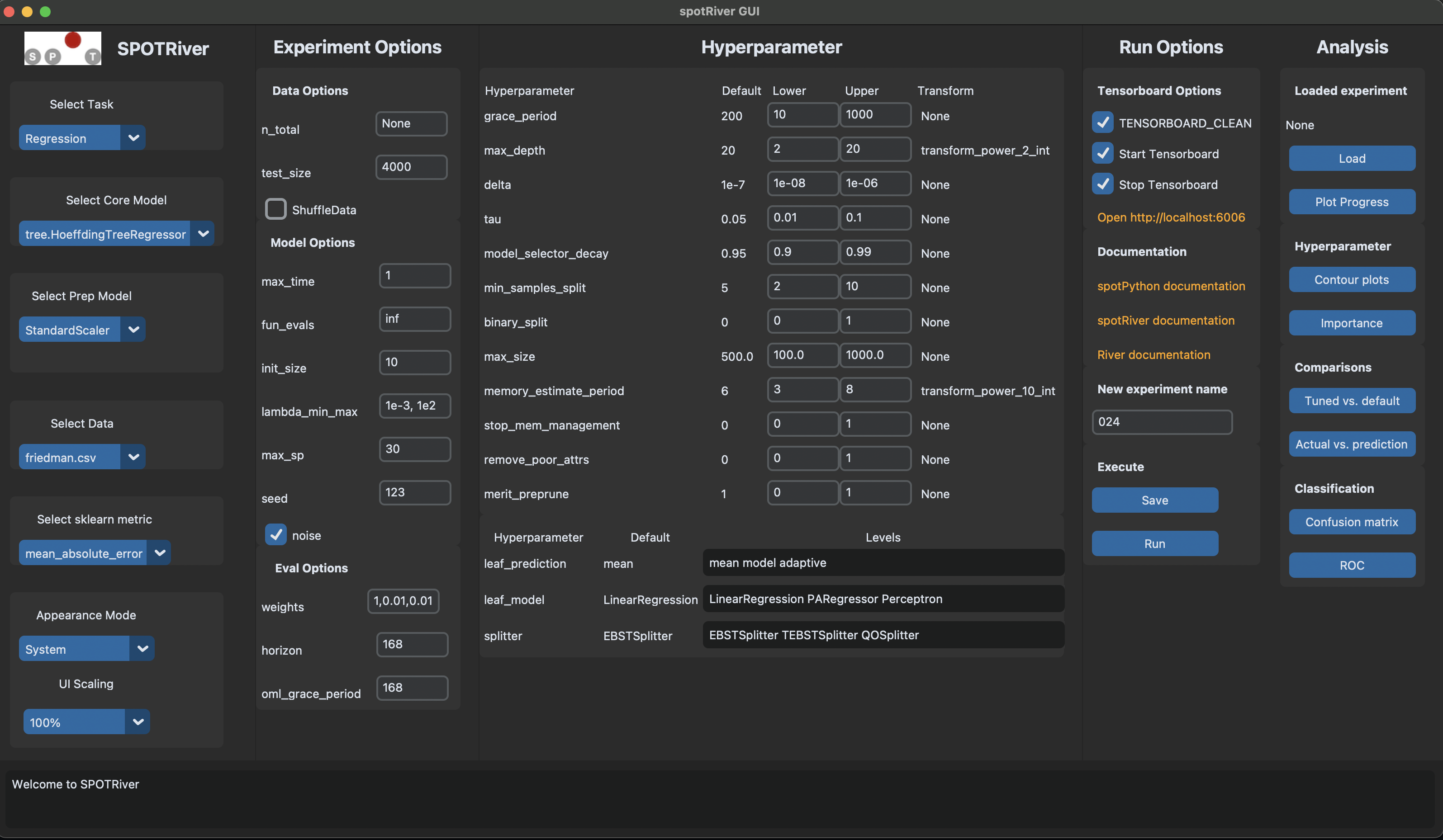
The spotgui [github] provides a convenient way to interact with the hyperparameter tuning process. To obtain the settings from Section 23.2.8, the spotgui can be started as shown in Figure 26.1.

23.4 Results

After the hyperparameter tuning run is finished, the progress of the hyperparameter tuning can be visualized with spotpython’s method plot_progress. The black points represent the performace values (score or metric) of hyperparameter configurations from the initial design, whereas the red points represents the hyperparameter configurations found by the surrogate model based optimization.

spot_tuner.plot_progress(log_y=True, filename=None)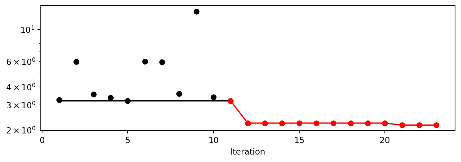

Results can be printed in tabular form.

from spotpython.utils.eda import gen_design_table
print(gen_design_table(fun_control=fun_control, spot=spot_tuner))

| name                   | type   | default          |   lower |   upper | tuned                 | transform              |   importance | stars   |
|------------------------|--------|------------------|---------|---------|-----------------------|------------------------|--------------|---------|
| grace_period           | int    | 200              |    10.0 |  1000.0 | 591.0                 | None                   |        20.87 | *       |
| max_depth              | int    | 20               |     2.0 |    20.0 | 2.0                   | transform_power_2_int  |         0.04 |         |
| delta                  | float  | 1e-07            |   1e-08 |   1e-06 | 4.994027045755513e-07 | None                   |        33.69 | *       |
| tau                    | float  | 0.05             |    0.01 |     0.1 | 0.04111324680641631   | None                   |         0.17 | .       |
| leaf_prediction        | factor | mean             |     0.0 |     2.0 | model                 | None                   |       100.00 | ***     |
| leaf_model             | factor | LinearRegression |     0.0 |     2.0 | LinearRegression      | None                   |         0.01 |         |
| model_selector_decay   | float  | 0.95             |     0.9 |    0.99 | 0.9551828562792138    | None                   |         3.11 | *       |
| splitter               | factor | EBSTSplitter     |     0.0 |     2.0 | QOSplitter            | None                   |         1.91 | *       |
| min_samples_split      | int    | 5                |     2.0 |    10.0 | 6.0                   | None                   |         0.31 | .       |
| binary_split           | factor | 0                |     0.0 |     1.0 | 1                     | None                   |         1.06 | *       |
| max_size               | float  | 500.0            |   100.0 |  1000.0 | 685.1800577726956     | None                   |         3.16 | *       |
| memory_estimate_period | int    | 6                |     3.0 |     8.0 | 4.0                   | transform_power_10_int |         0.00 |         |
| stop_mem_management    | factor | 0                |     0.0 |     1.0 | 1                     | None                   |         0.04 |         |
| remove_poor_attrs      | factor | 0                |     0.0 |     1.0 | 0                     | None                   |         0.09 |         |
| merit_preprune         | factor | 1                |     0.0 |     1.0 | 0                     | None                   |         0.02 |         |

A histogram can be used to visualize the most important hyperparameters.

spot_tuner.plot_importance(threshold=10.0)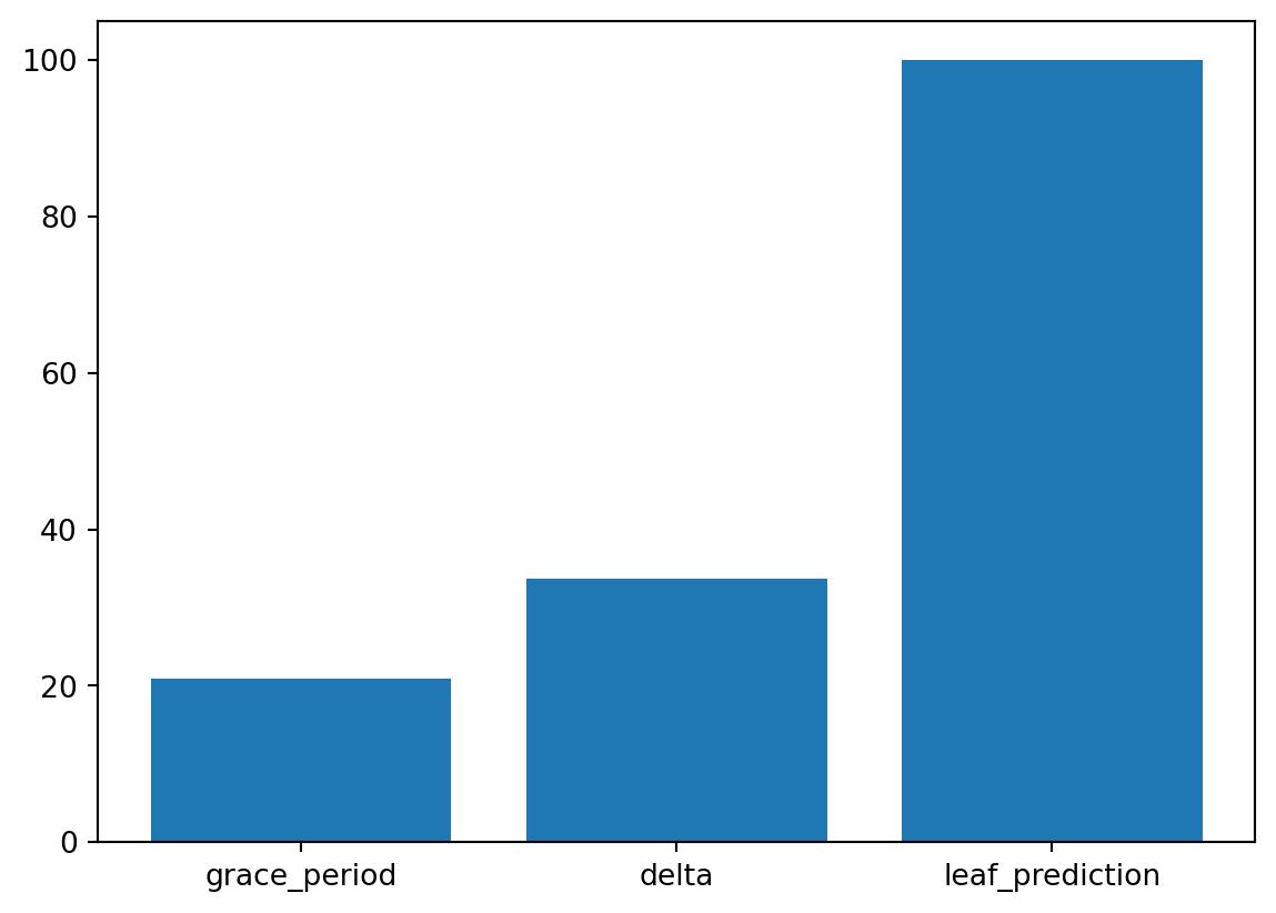

23.5 Performance of the Model with Default Hyperparameters

23.5.1 Get Default Hyperparameters and Fit the Model

The default hyperparameters, which will be used for a comparion with the tuned hyperparameters, can be obtained with the following commands:

from spotpython.hyperparameters.values import get_default_hyperparameters_as_array
X_start = get_default_hyperparameters_as_array(fun_control)

spotpython tunes numpy arrays, i.e., the hyperparameters are stored in a numpy array.

from spotpython.hyperparameters.values import get_one_core_model_from_X
model_default = get_one_core_model_from_X(X_start, fun_control, default=True)

23.5.2 Evaluate the Model with Default Hyperparameters

The model with the default hyperparameters can be trained and evaluated. The evaluation function eval_oml_horizon [SOURCE] is the same function that was used for the hyperparameter tuning. During the hyperparameter tuning, the evaluation function was called from the objective (or loss) function fun_oml_horizon [SOURCE].

from spotriver.evaluation.eval_bml import eval_oml_horizon

df_eval_default, df_true_default = eval_oml_horizon(
                    model=model_default,
                    train=fun_control["train"],
                    test=fun_control["test"],
                    target_column=fun_control["target_column"],
                    horizon=fun_control["horizon"],
                    oml_grace_period=fun_control["oml_grace_period"],
                    metric=fun_control["metric_sklearn"],
                )

The three performance criteria, i.e., score (metric), runtime, and memory consumption, can be visualized with the following commands:

from spotriver.evaluation.eval_bml import plot_bml_oml_horizon_metrics, plot_bml_oml_horizon_predictions
df_labels=["default"]
plot_bml_oml_horizon_metrics(df_eval = [df_eval_default], log_y=False, df_labels=df_labels, metric=fun_control["metric_sklearn"])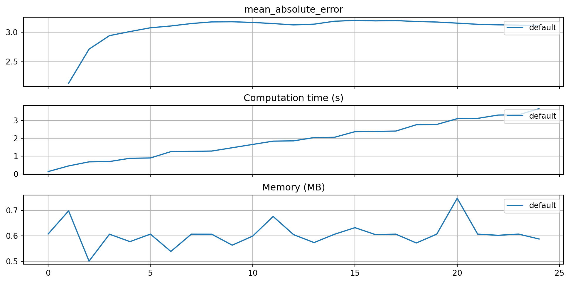

23.5.3 Show Predictions of the Model with Default Hyperparameters

Select a subset of the data set for the visualization of the predictions:
- We use the mean, \(m\), of the data set as the center of the visualization.
- We use 100 data points, i.e., \(m \pm 50\) as the visualization window.

m = fun_control["test"].shape[0]
a = int(m/2)-50
b = int(m/2)+50
plot_bml_oml_horizon_predictions(df_true = [df_true_default[a:b]], target_column=target_column,  df_labels=df_labels)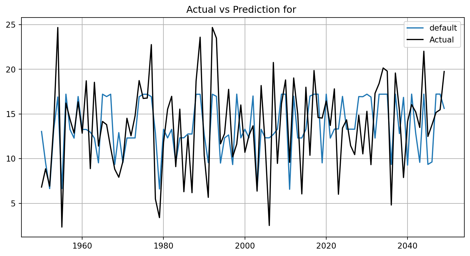

23.6 Get SPOT Results

In a similar way, we can obtain the hyperparameters found by spotpython.

from spotpython.hyperparameters.values import get_one_core_model_from_X
X = spot_tuner.to_all_dim(spot_tuner.min_X.reshape(1,-1))
model_spot = get_one_core_model_from_X(X, fun_control)

df_eval_spot, df_true_spot = eval_oml_horizon(
                    model=model_spot,
                    train=fun_control["train"],
                    test=fun_control["test"],
                    target_column=fun_control["target_column"],
                    horizon=fun_control["horizon"],
                    oml_grace_period=fun_control["oml_grace_period"],
                    metric=fun_control["metric_sklearn"],
                )

df_labels=["default", "spot"]
plot_bml_oml_horizon_metrics(df_eval = [df_eval_default, df_eval_spot], log_y=False, df_labels=df_labels, metric=fun_control["metric_sklearn"])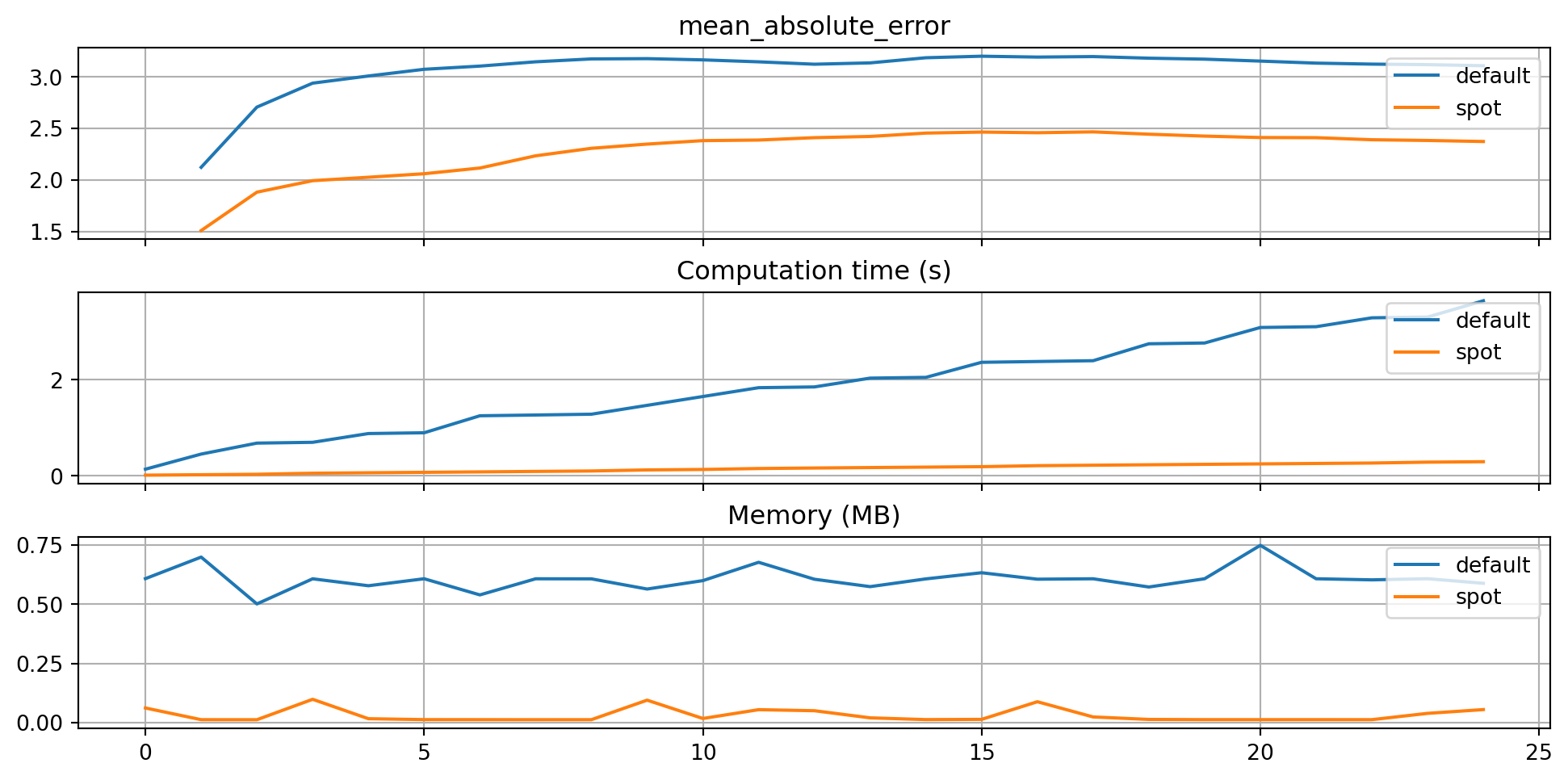

plot_bml_oml_horizon_predictions(df_true = [df_true_default[a:b], df_true_spot[a:b]], target_column=target_column,  df_labels=df_labels)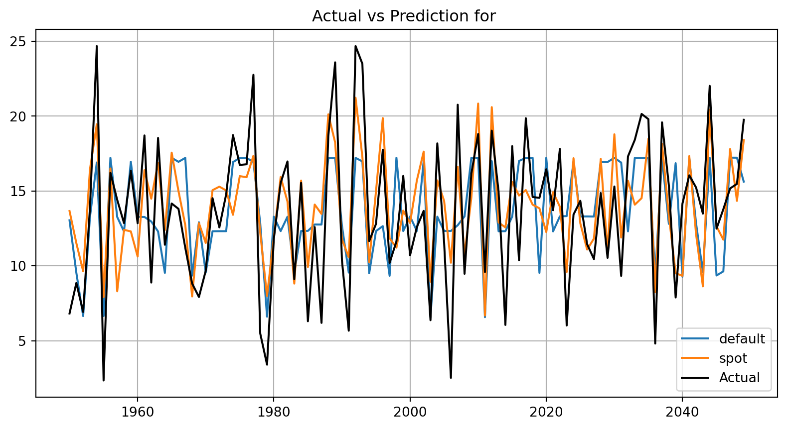

from spotpython.plot.validation import plot_actual_vs_predicted
plot_actual_vs_predicted(y_test=df_true_default[target_column], y_pred=df_true_default["Prediction"], title="Default")
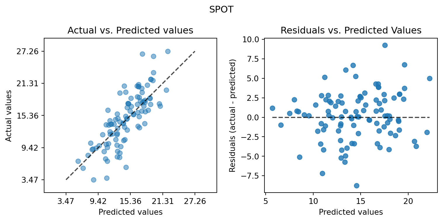
plot_actual_vs_predicted(y_test=df_true_spot[target_column], y_pred=df_true_spot["Prediction"], title="SPOT")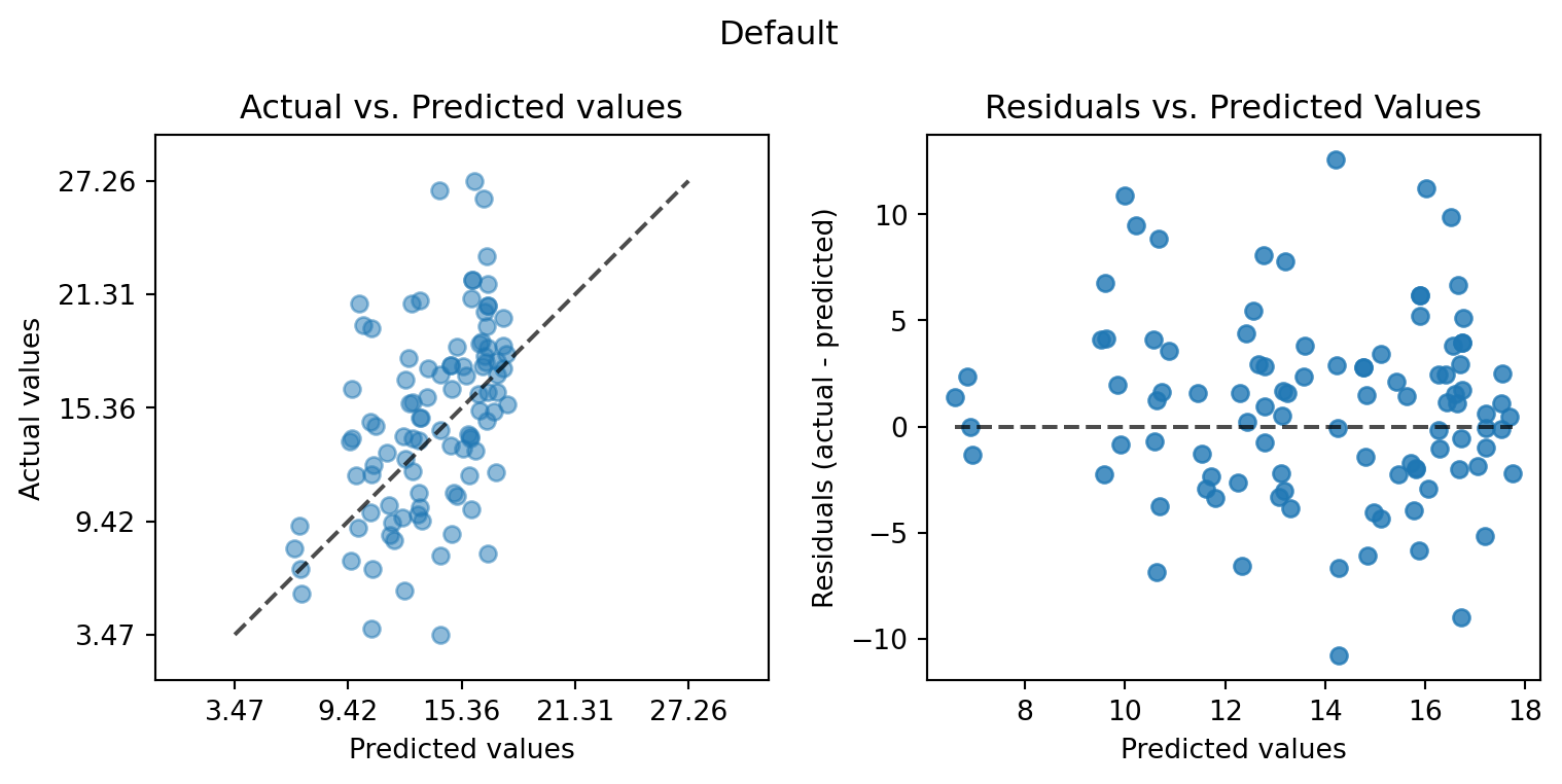

23.7 Visualize Regression Trees

dataset_f = dataset.take(n_samples)
print(f"n_samples: {n_samples}")
for x, y in dataset_f:
    model_default.learn_one(x, y)

n_samples: 10000

Caution: Large Trees

Since the trees are large, the visualization is suppressed by default.
To visualize the trees, uncomment the following line.

# model_default.draw()

model_default.summary

{'n_nodes': 23,
 'n_branches': 11,
 'n_leaves': 12,
 'n_active_leaves': 12,
 'n_inactive_leaves': 0,
 'height': 7,
 'total_observed_weight': 14168.0}

23.7.1 Spot Model

print(f"n_samples: {n_samples}")
dataset_f = dataset.take(n_samples)
for x, y in dataset_f:
    model_spot.learn_one(x, y)

n_samples: 10000

Caution: Large Trees

Since the trees are large, the visualization is suppressed by default.
To visualize the trees, uncomment the following line.

# model_spot.draw()

model_spot.summary

{'n_nodes': 11,
 'n_branches': 5,
 'n_leaves': 6,
 'n_active_leaves': 4,
 'n_inactive_leaves': 2,
 'height': 5,
 'total_observed_weight': 14168.0}

from spotpython.utils.eda import compare_two_tree_models
print(compare_two_tree_models(model_default, model_spot))

| Parameter             |   Default |   Spot |
|-----------------------|-----------|--------|
| n_nodes               |        23 |     11 |
| n_branches            |        11 |      5 |
| n_leaves              |        12 |      6 |
| n_active_leaves       |        12 |      4 |
| n_inactive_leaves     |         0 |      2 |
| height                |         7 |      5 |
| total_observed_weight |     14168 |  14168 |

23.8 Detailed Hyperparameter Plots

spot_tuner.plot_important_hyperparameter_contour(max_imp=3)

grace_period:  20.873139039731644
max_depth:  0.03511587880120552
delta:  33.69309470902903
tau:  0.1679770885200379
leaf_prediction:  100.0
leaf_model:  0.006846012567192482
model_selector_decay:  3.1056711928301426
splitter:  1.9103105617533682
min_samples_split:  0.31151861155710786
binary_split:  1.0635492633913082
max_size:  3.1639735224217698
memory_estimate_period:  0.003630545866184321
stop_mem_management:  0.03606141484237544
remove_poor_attrs:  0.09174212775479652
merit_preprune:  0.018082433169196704

23.9 Parallel Coordinates Plots

spot_tuner.parallel_plot()

23.1 The Friedman Drift Data Set

23.2 Setup

23.2.1 General Experiment Setup

23.2.2 Data Setup

23.2.3 Evaluation Setup

23.2.4 River-Specific Setup

23.2.5 Model Setup

23.2.6 Objective Function Setup

23.2.7 Surrogate Model Setup

23.2.8 Summary: Setting up the Experiment

23.2.9 Run the Spot Optimizer

23.3 Using the spotgui

23.4 Results

23.5 Performance of the Model with Default Hyperparameters

23.5.1 Get Default Hyperparameters and Fit the Model

23.5.2 Evaluate the Model with Default Hyperparameters

23.5.3 Show Predictions of the Model with Default Hyperparameters

23.6 Get SPOT Results

23.7 Visualize Regression Trees

23.7.1 Spot Model

23.8 Detailed Hyperparameter Plots

23.9 Parallel Coordinates Plots

23.2.9 Run the `Spot` Optimizer

23.3 Using the `spotgui`