import numpy as np
from math import inf
from spotpython.fun.objectivefunctions import Analytical
from spotpython.spot import Spot
from spotpython.utils.init import fun_control_init, surrogate_control_init
PREFIX="015"21 Kriging with Varying Correlation-p
This chapter illustrates the difference between Kriging models with varying p. The difference is illustrated with the help of the spotpython package.
21.1 Example: Spot Surrogate and the 2-dim Sphere Function
21.1.1 The Objective Function: 2-dim Sphere
- The
spotpythonpackage provides several classes of objective functions. - We will use an analytical objective function, i.e., a function that can be described by a (closed) formula: \[f(x, y) = x^2 + y^2\]
- The size of the
lowerbound vector determines the problem dimension. - Here we will use
np.array([-1, -1]), i.e., a two-dim function.
fun = Analytical().fun_sphere
fun_control = fun_control_init(PREFIX=PREFIX,
                               lower = np.array([-1, -1]),
upper = np.array([1, 1]))- Although the default
spotsurrogate model is an isotropic Kriging model, we will explicitly set thethetaparameter to a value of1for both dimensions. This is done to illustrate the difference between isotropic and anisotropic Kriging models.
surrogate_control=surrogate_control_init(n_p=1,
                                         p_val=2.0,)
spot_2 = Spot(fun=fun,
fun_control=fun_control,
surrogate_control=surrogate_control)
spot_2.run()spotpython tuning: 6.611333241687761e-06 [#######---] 73.33%. Success rate: 100.00%
spotpython tuning: 6.611333241687761e-06 [########--] 80.00%. Success rate: 50.00%
spotpython tuning: 6.611333241687761e-06 [#########-] 86.67%. Success rate: 33.33%
spotpython tuning: 6.611333241687761e-06 [#########-] 93.33%. Success rate: 25.00%
spotpython tuning: 3.1531067682958562e-06 [##########] 100.00%. Success rate: 40.00% Done...
Experiment saved to 015_res.pkl<spotpython.spot.spot.Spot at 0x1047cc050>21.1.2 Results
spot_2.print_results()min y: 3.1531067682958562e-06
x0: -0.0012459503825024937
x1: -0.0012651934289418935[['x0', np.float64(-0.0012459503825024937)],
['x1', np.float64(-0.0012651934289418935)]]spot_2.plot_progress(log_y=True)
spot_2.surrogate.plot()
21.2 Example With Modified p
- We can use set
p_valto a value other than2to obtain a different Kriging model.
surrogate_control = surrogate_control_init(n_p=1,
                                           p_val=1.0)
spot_2_p1= Spot(fun=fun,
                    fun_control=fun_control,
                    surrogate_control=surrogate_control)
spot_2_p1.run()
spotpython tuning: 6.611333241687761e-06 [#######---] 73.33%. Success rate: 100.00%
spotpython tuning: 6.611333241687761e-06 [########--] 80.00%. Success rate: 50.00%
spotpython tuning: 6.611333241687761e-06 [#########-] 86.67%. Success rate: 33.33%
spotpython tuning: 6.611333241687761e-06 [#########-] 93.33%. Success rate: 25.00%
spotpython tuning: 3.1531067682958562e-06 [##########] 100.00%. Success rate: 40.00% Done...
Experiment saved to 015_res.pkl<spotpython.spot.spot.Spot at 0x1542cb750>- The search progress of the optimization with the anisotropic model can be visualized:
spot_2_p1.plot_progress(log_y=True)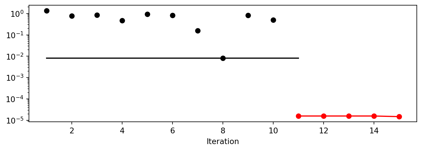
spot_2_p1.print_results()min y: 3.1531067682958562e-06
x0: -0.0012459503825024937
x1: -0.0012651934289418935[['x0', np.float64(-0.0012459503825024937)],
['x1', np.float64(-0.0012651934289418935)]]spot_2_p1.surrogate.plot()
21.2.1 Taking a Look at the p_val Values
21.2.1.1 p_val Values from the spot Model
- We can check, which
p_valvalues thespotmodel has used: - The
p_valvalues from the surrogate can be printed as follows:
spot_2_p1.surrogate.p_val1.0- Since the surrogate from the isotropic setting was stored as
spot_2, we can also take a look at thethetavalue from this model:
spot_2.surrogate.p_val2.021.3 Optimization of the p_val Values
surrogate_control = surrogate_control_init(n_p=1,
                                           optim_p=True)
spot_2_pm= Spot(fun=fun,
                    fun_control=fun_control,
                    surrogate_control=surrogate_control)
spot_2_pm.run()
spotpython tuning: 6.5058325242694635e-06 [#######---] 73.33%. Success rate: 100.00%
spotpython tuning: 6.5058325242694635e-06 [########--] 80.00%. Success rate: 50.00%
spotpython tuning: 6.5058325242694635e-06 [#########-] 86.67%. Success rate: 33.33%
spotpython tuning: 6.5058325242694635e-06 [#########-] 93.33%. Success rate: 25.00%
spotpython tuning: 4.326910928440869e-06 [##########] 100.00%. Success rate: 40.00% Done...
Experiment saved to 015_res.pkl<spotpython.spot.spot.Spot at 0x156fefed0>spot_2_pm.plot_progress(log_y=True)
spot_2_pm.print_results()min y: 4.326910928440869e-06
x0: -0.0018878035376713096
x1: -0.0008735609489878526[['x0', np.float64(-0.0018878035376713096)],
['x1', np.float64(-0.0008735609489878526)]]spot_2_pm.surrogate.plot()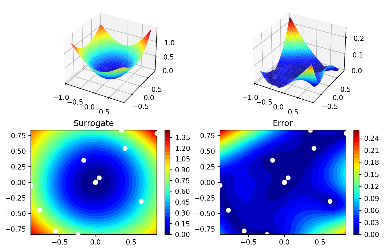
spot_2_pm.surrogate.p_valarray([1.44960552])21.4 Optimization of Multiple p_val Values
surrogate_control = surrogate_control_init(n_p=2,
                                           optim_p=True)
spot_2_pmo= Spot(fun=fun,
                    fun_control=fun_control,
                    surrogate_control=surrogate_control)
spot_2_pmo.run()
spotpython tuning: 8.652107435275436e-06 [#######---] 73.33%. Success rate: 100.00%
spotpython tuning: 8.652107435275436e-06 [########--] 80.00%. Success rate: 50.00%
spotpython tuning: 8.652107435275436e-06 [#########-] 86.67%. Success rate: 33.33%
spotpython tuning: 8.652107435275436e-06 [#########-] 93.33%. Success rate: 25.00%
spotpython tuning: 8.652107435275436e-06 [##########] 100.00%. Success rate: 20.00% Done...
Experiment saved to 015_res.pkl<spotpython.spot.spot.Spot at 0x1545a0a50>spot_2_pmo.plot_progress(log_y=True)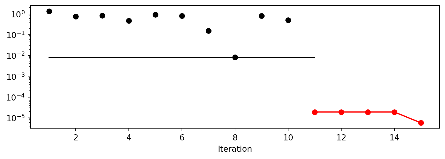
spot_2_pmo.print_results()min y: 8.652107435275436e-06
x0: 0.0006053414964068362
x1: 0.002878483821042489[['x0', np.float64(0.0006053414964068362)],
['x1', np.float64(0.002878483821042489)]]spot_2_pmo.surrogate.plot()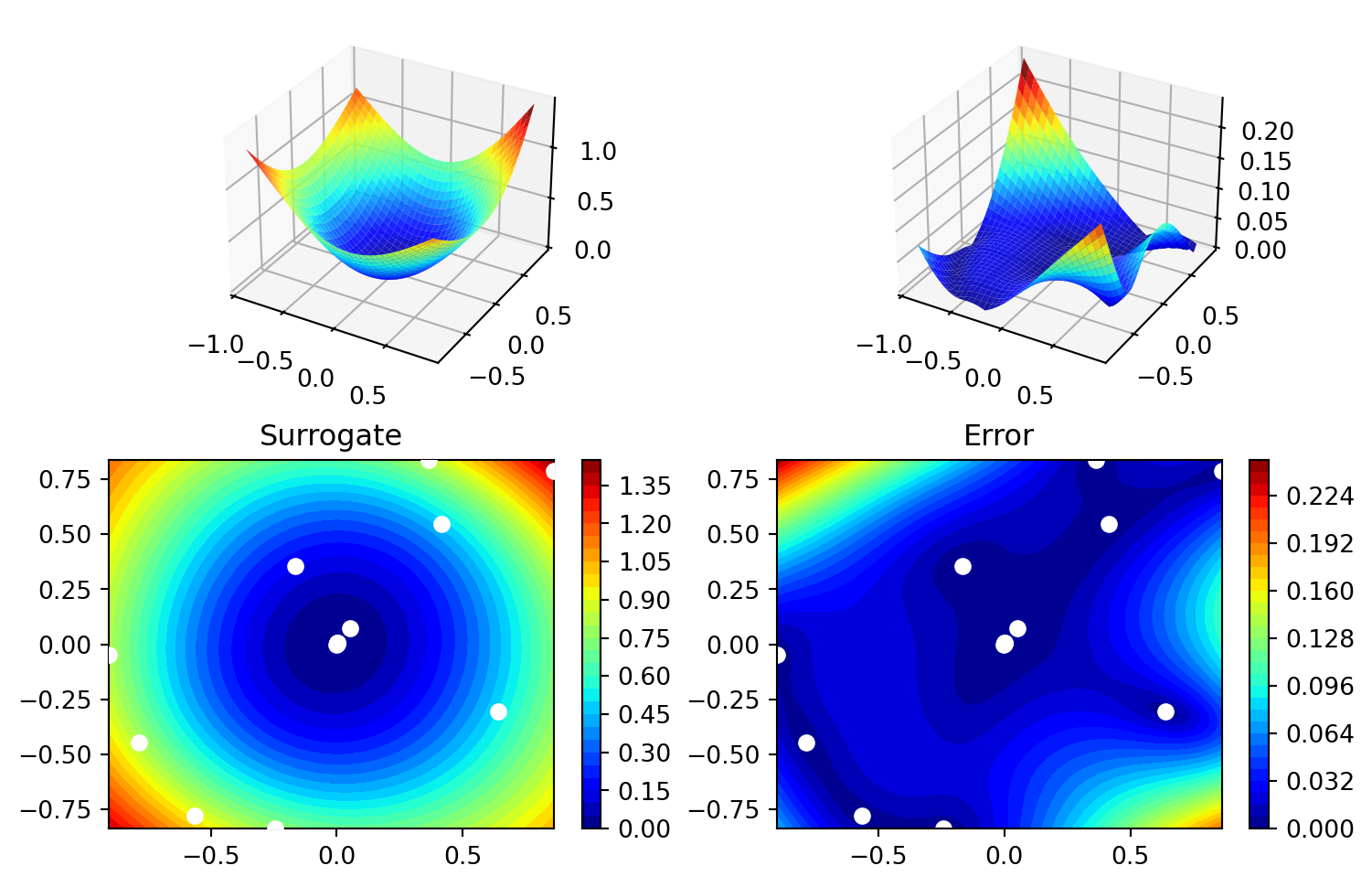
spot_2_pmo.surrogate.p_valarray([1.61192933, 1.76827516])21.5 Exercises
21.5.1 fun_branin
- Describe the function.
- The input dimension is
2. The search range is \(-5 \leq x_1 \leq 10\) and \(0 \leq x_2 \leq 15\).
- The input dimension is
- Compare the results from
spotpythonruns with different options forp_val. - Modify the termination criterion: instead of the number of evaluations (which is specified via
fun_evals), the time should be used as the termination criterion. This can be done as follows (max_time=1specifies a run time of one minute):
fun_evals=inf,
max_time=1,
21.5.2 fun_sin_cos
- Describe the function.
- The input dimension is
2. The search range is \(-2\pi \leq x_1 \leq 2\pi\) and \(-2\pi \leq x_2 \leq 2\pi\).
- The input dimension is
- Compare the results from
spotpythonrun a) with isotropic and b) anisotropic surrogate models. - Modify the termination criterion (
max_timeinstead offun_evals) as described forfun_branin.
21.5.3 fun_runge
- Describe the function.
- The input dimension is
2. The search range is \(-5 \leq x_1 \leq 5\) and \(-5 \leq x_2 \leq 5\).
- The input dimension is
- Compare the results from
spotpythonruns with different options forp_val. - Modify the termination criterion (
max_timeinstead offun_evals) as described forfun_branin.
21.5.4 fun_wingwt
- Describe the function.
- The input dimension is
10. The search ranges are between 0 and 1 (values are mapped internally to their natural bounds).
- The input dimension is
- Compare the results from
spotpythonruns with different options forp_val. - Modify the termination criterion (
max_timeinstead offun_evals) as described forfun_branin.
21.6 Jupyter Notebook
Note
- The Jupyter-Notebook of this lecture is available on GitHub in the Hyperparameter-Tuning-Cookbook Repository