import numpy as np
from math import inf
from spotpython.fun.objectivefunctions import Analytical
from spotpython.spot import Spot
from spotpython.utils.init import fun_control_init, surrogate_control_init
PREFIX="003"14 Isotropic and Anisotropic Kriging
This chapter illustrates the difference between isotropic and anisotropic Kriging models. The difference is illustrated with the help of the spotpython package. Isotropic Kriging models use the same theta value for every dimension. Anisotropic Kriging models use different theta values for each dimension.
14.1 Example: Isotropic Spot Surrogate and the 2-dim Sphere Function
14.1.1 The Objective Function: 2-dim Sphere
The spotpython package provides several classes of objective functions. We will use an analytical objective function, i.e., a function that can be described by a (closed) formula:
\[
f(x, y) = x^2 + y^2
\] The size of the lower bound vector determines the problem dimension. Here we will use np.array([-1, -1]), i.e., a two-dimensional function.
fun = Analytical().fun_sphere
fun_control = fun_control_init(PREFIX=PREFIX,
                               lower = np.array([-1, -1]),
                               upper = np.array([1, 1]))
The default Spot surrogate model is an anisotropic Kriging model. We will explicitly set the isotropic parameter to a value of False, so that the same theta value is used for both dimensions. This is done to illustrate the difference between isotropic and anisotropic Kriging models.
surrogate_control=surrogate_control_init(isotropic=True)spot_2 = Spot(fun=fun,
fun_control=fun_control,
surrogate_control=surrogate_control)
spot_2.run()spotpython tuning: 0.0025690995161869214 [#######---] 73.33%. Success rate: 100.00%
spotpython tuning: 0.0025690995161869214 [########--] 80.00%. Success rate: 50.00%
spotpython tuning: 0.0025690995161869214 [#########-] 86.67%. Success rate: 33.33%
spotpython tuning: 0.0025690995161869214 [#########-] 93.33%. Success rate: 25.00%
spotpython tuning: 0.0025690995161869214 [##########] 100.00%. Success rate: 20.00% Done...
Experiment saved to 003_res.pkl<spotpython.spot.spot.Spot at 0x106a34050>14.1.2 Results
spot_2.print_results()min y: 0.0025690995161869214
x0: 0.03166420094465901
x1: 0.03957875559846692[['x0', np.float64(0.03166420094465901)],
['x1', np.float64(0.03957875559846692)]]spot_2.plot_progress(log_y=True)
14.2 Example With Anisotropic Kriging
As described in Section 14.1, the default parameter setting of spotpython’s Kriging surrogate uses different theta value for every dimension. This is referred to as “using an anisotropic kernel”. To enable isotropic models in spotpython, the command surrogate_control=surrogate_control_init(isotropic=True) can be used. In this case, the same theta value is used for every dimension.
spot_2_anisotropic = Spot(fun=fun,
                    fun_control=fun_control)
spot_2_anisotropic.run()
spotpython tuning: 6.611333241687761e-06 [#######---] 73.33%. Success rate: 100.00%
spotpython tuning: 6.611333241687761e-06 [########--] 80.00%. Success rate: 50.00%
spotpython tuning: 6.611333241687761e-06 [#########-] 86.67%. Success rate: 33.33%
spotpython tuning: 6.611333241687761e-06 [#########-] 93.33%. Success rate: 25.00%
spotpython tuning: 3.1531067682958562e-06 [##########] 100.00%. Success rate: 40.00% Done...
Experiment saved to 003_res.pkl<spotpython.spot.spot.Spot at 0x154ccb750>The search progress of the optimization with the anisotropic model can be visualized:
spot_2_anisotropic.plot_progress(log_y=True)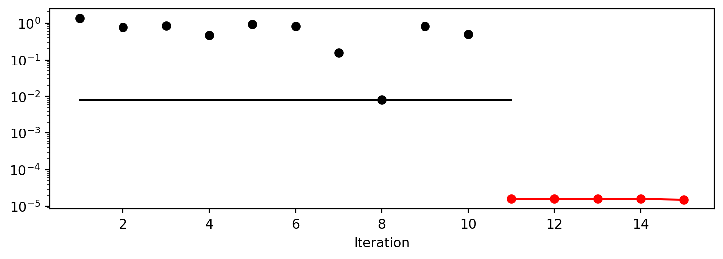
spot_2_anisotropic.print_results()min y: 3.1531067682958562e-06
x0: -0.0012459503825024937
x1: -0.0012651934289418935[['x0', np.float64(-0.0012459503825024937)],
['x1', np.float64(-0.0012651934289418935)]]spot_2_anisotropic.surrogate.plot()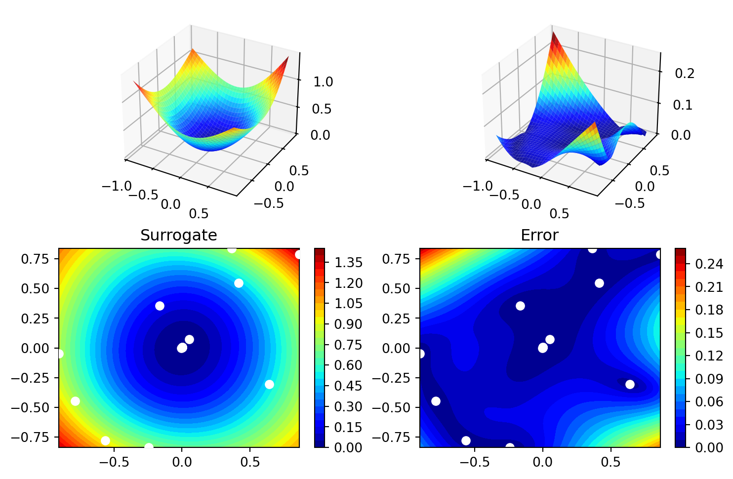
14.2.1 Taking a Look at the theta Values
14.2.1.1 theta Values from the spot Model
We can check, whether one or several theta values were used. The theta values from the surrogate can be printed as follows:
spot_2_anisotropic.surrogate.thetaarray([-0.35825091, -0.1916896 ])- Since the surrogate from the isotropic setting was stored as
spot_2, we can also take a look at thethetavalue from this model:
spot_2.surrogate.thetaarray([-0.07437973])14.2.1.2 TensorBoard
Now we can start TensorBoard in the background with the following command:
tensorboard --logdir="./runs"We can access the TensorBoard web server with the following URL:
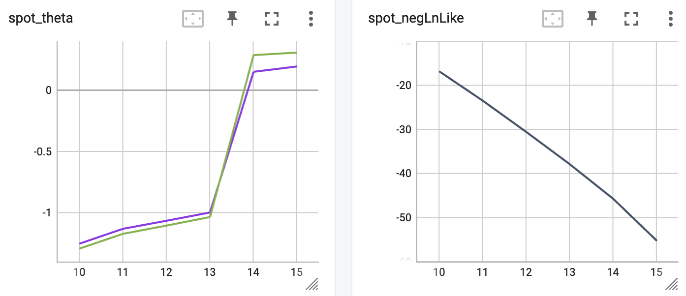
http://localhost:6006/The TensorBoard plot illustrates how spotpython can be used as a microscope for the internal mechanisms of the surrogate-based optimization process. Here, one important parameter, the learning rate \(\theta\) of the Kriging surrogate is plotted against the number of optimization steps.
14.3 Exercises
14.3.1 1. The Branin Function fun_branin
- Describe the function.
- The input dimension is
2. The search range is \(-5 \leq x_1 \leq 10\) and \(0 \leq x_2 \leq 15\).
- The input dimension is
- Compare the results from
spotpythonrun a) with isotropic and b) anisotropic surrogate models. - Modify the termination criterion: instead of the number of evaluations (which is specified via
fun_evals), the time should be used as the termination criterion. This can be done as follows (max_time=1specifies a run time of one minute):
from math import inf
fun_control = fun_control_init(
              fun_evals=inf,
              max_time=1)
14.3.2 2. The Two-dimensional Sin-Cos Function fun_sin_cos
- Describe the function.
- The input dimension is
2. The search range is \(-2\pi \leq x_1 \leq 2\pi\) and \(-2\pi \leq x_2 \leq 2\pi\).
- The input dimension is
- Compare the results from
spotpythonrun a) with isotropic and b) anisotropic surrogate models. - Modify the termination criterion (
max_timeinstead offun_evals) as described forfun_branin.
14.3.3 3. The Two-dimensional Runge Function fun_runge
- Describe the function.
- The input dimension is
2. The search range is \(-5 \leq x_1 \leq 5\) and \(-5 \leq x_2 \leq 5\).
- The input dimension is
- Compare the results from
spotpythonrun a) with isotropic and b) anisotropic surrogate models. - Modify the termination criterion (
max_timeinstead offun_evals) as described forfun_branin.
14.3.4 4. The Ten-dimensional Wing-Weight Function fun_wingwt
- Describe the function.
- The input dimension is
10. The search ranges are between 0 and 1 (values are mapped internally to their natural bounds).
- The input dimension is
- Compare the results from
spotpythonrun a) with isotropic and b) anisotropic surrogate models. - Modify the termination criterion (
max_timeinstead offun_evals) as described forfun_branin.
14.3.5 5. The Two-dimensional Rosenbrock Function fun_rosen
- Describe the function.
- The input dimension is
2. The search ranges are between -5 and 10.
- The input dimension is
- Compare the results from
spotpythonrun a) with isotropic and b) anisotropic surrogate models. - Modify the termination criterion (
max_timeinstead offun_evals) as described forfun_branin.
14.4 Selected Solutions
14.4.1 Solution to Exercise Section 14.3.5: The Two-dimensional Rosenbrock Function fun_rosen
14.4.1.1 The Two Dimensional fun_rosen: The Isotropic Case
import numpy as np
from spotpython.fun.objectivefunctions import Analytical
from spotpython.utils.init import fun_control_init, surrogate_control_init
from spotpython.spot import Spot
The spotpython package provides several classes of objective functions. We will use the fun_rosen in the analytical class [SOURCE].
fun_rosen = Analytical().fun_rosenHere we will use problem dimension \(k=2\), which can be specified by the lower bound arrays. The size of the lower bound array determines the problem dimension.
The prefix is set to "ROSEN" to distinguish the results from the one-dimensional case. Again, TensorBoard can be used to monitor the progress of the optimization.
fun_control = fun_control_init(
              PREFIX="ROSEN",
              lower = np.array([-5, -5]),
              upper = np.array([10, 10]),
              show_progress=True)
surrogate_control = surrogate_control_init(isotropic=True)
spot_rosen = Spot(fun=fun_rosen,
                  fun_control=fun_control,
                  surrogate_control=surrogate_control)
spot_rosen.run()
spotpython tuning: 53.73873931238049 [#######---] 73.33%. Success rate: 100.00%
spotpython tuning: 49.866300631713166 [########--] 80.00%. Success rate: 100.00%
spotpython tuning: 49.866300631713166 [#########-] 86.67%. Success rate: 66.67%
spotpython tuning: 12.621648163047155 [#########-] 93.33%. Success rate: 75.00%
spotpython tuning: 12.621648163047155 [##########] 100.00%. Success rate: 60.00% Done...
Experiment saved to ROSEN_res.pkl<spotpython.spot.spot.Spot at 0x156720690>
Note
Now we can start TensorBoard in the background with the following command:
tensorboard --logdir="./runs"and can access the TensorBoard web server with the following URL:
http://localhost:6006/14.4.1.1.1 Results
_ = spot_rosen.print_results()min y: 12.621648163047155
x0: -0.5398890007511357
x1: -0.7209619653808784spot_rosen.plot_progress()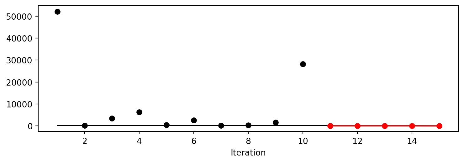
14.4.1.1.2 A Contour Plot
We can select two dimensions, say \(i=0\) and \(j=1\), and generate a contour plot as follows.
min_z = None
max_z = None
spot_rosen.plot_contour(i=0, j=1, min_z=min_z, max_z=max_z)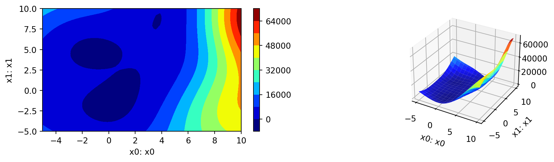
- The variable importance cannot be calculated, because only one
thetavalue was used.
14.4.1.1.3 TensorBoard
TBD
14.4.1.2 The Two Dimensional fun_rosen: The Anisotropic Case
import numpy as np
from spotpython.fun.objectivefunctions import Analytical
from spotpython.utils.init import fun_control_init, surrogate_control_init
from spotpython.spot import Spot
The spotpython package provides several classes of objective functions. We will use the fun_rosen in the analytical class [SOURCE].
fun_rosen = Analytical().fun_rosenHere we will use problem dimension \(k=2\), which can be specified by the lower bound arrays. The size of the lower bound array determines the problem dimension. The default anisotropic kernel is used, so no isotropic parameter is set.
We can also add interpretable labels to the dimensions, which will be used in the plots.
fun_control = fun_control_init(
              PREFIX="ROSEN",
              lower = np.array([-5, -5]),
              upper = np.array([10, 10]),
              show_progress=True)
spot_rosen = Spot(fun=fun_rosen,
                  fun_control=fun_control)
spot_rosen.run()
spotpython tuning: 90.77788110350957 [#######---] 73.33%. Success rate: 100.00%
spotpython tuning: 1.0173064877521703 [########--] 80.00%. Success rate: 100.00%
spotpython tuning: 1.0173064877521703 [#########-] 86.67%. Success rate: 66.67%
spotpython tuning: 1.0173064877521703 [#########-] 93.33%. Success rate: 50.00%
spotpython tuning: 0.7867277329036355 [##########] 100.00%. Success rate: 60.00% Done...
Experiment saved to ROSEN_res.pkl<spotpython.spot.spot.Spot at 0x156720410>
Note
Now we can start TensorBoard in the background with the following command:
tensorboard --logdir="./runs"and can access the TensorBoard web server with the following URL:
http://localhost:6006/14.4.1.2.1 Results
_ = spot_rosen.print_results()min y: 0.7867277329036355
x0: 0.13953655588708272
x1: 0.08753688433642533spot_rosen.plot_progress()
14.4.1.2.2 A Contour Plot
We can select two dimensions, say \(i=0\) and \(j=1\), and generate a contour plot as follows.
min_z = None
max_z = None
spot_rosen.plot_contour(i=0, j=1, min_z=min_z, max_z=max_z)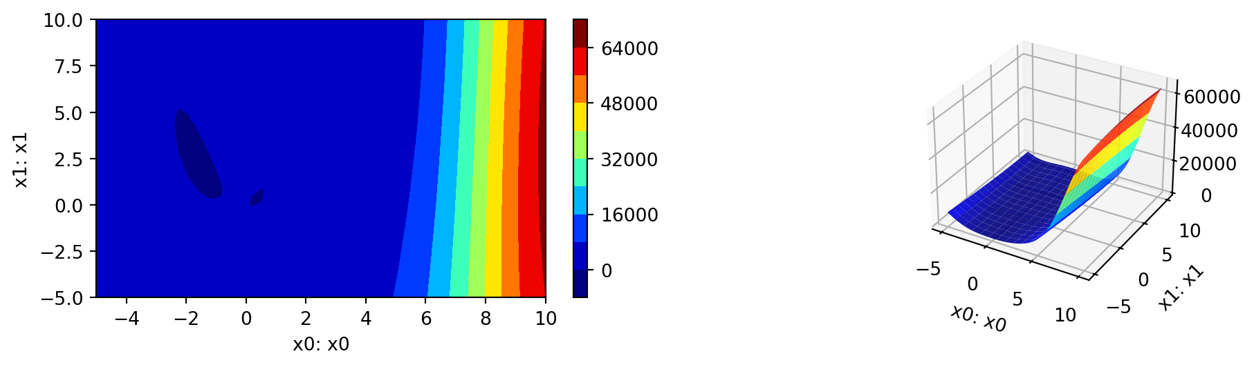
- The variable importance can be calculated as follows:
_ = spot_rosen.print_importance()x0: 100.0
x1: 2.8374127215640144spot_rosen.plot_importance()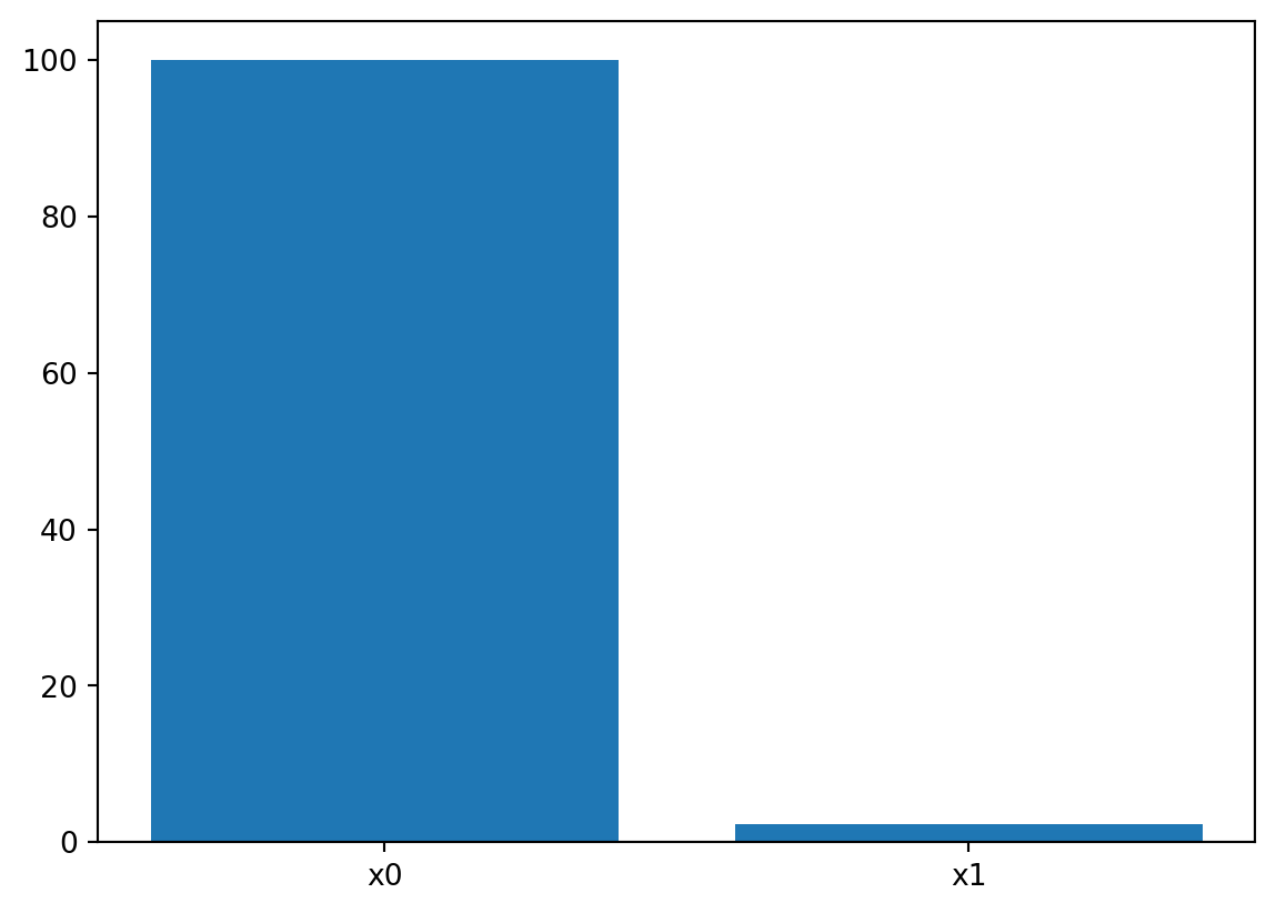
14.4.1.2.3 TensorBoard
TBD
14.5 Jupyter Notebook
Note
- The Jupyter-Notebook of this lecture is available on GitHub in the Hyperparameter-Tuning-Cookbook Repository