import time
from math import inf
import multiprocessing
import matplotlib.pyplot as plt
import pandas as pd
import numpy as np
from spotpython.data.diabetes import Diabetes
from spotpython.hyperdict.light_hyper_dict import LightHyperDict
from spotpython.fun.hyperlight import HyperLight
from spotpython.utils.init import (fun_control_init, design_control_init)
from spotpython.hyperparameters.values import set_hyperparameter
from spotpython.spot import Spot
from spotpython.utils.parallel import make_parallelAppendix H — Parallelism in Initial Design
In spotpython, we provide a wrapper function, that encapsulates the objective function to enable its parallel execution via multiprocessing or joblib, allowing multiple configurations to be evaluated at the same time.
H.1 Setup
To demonstrate the performance gain enabled by parallelization, we use a similar example to that in Section 47, where we perform hyperparameter tuning with spotpythonand PyTorch Lightning on the Diabetes dataset using a ResNet model. We compare the time required with and without parallelization. First, we import the necessary libraries, including the wrapper function make_parallel. We then define the fun_control and design_control settings. For design_control, we deliberately choose an initial design size of 10 for demonstration purposes.
dataset = Diabetes()
fun_control = fun_control_init(
    fun_evals=10,
    max_time=inf,
    data_set=dataset,
    core_model_name="light.regression.NNResNetRegressor",
    hyperdict=LightHyperDict,
    _L_in=10,
    _L_out=1,
    seed=125,
    tensorboard_log=False,
    TENSORBOARD_CLEAN=False,
)
set_hyperparameter(fun_control, "optimizer", ["Adadelta", "Adam", "Adamax"])
set_hyperparameter(fun_control, "l1", [2, 5])
set_hyperparameter(fun_control, "epochs", [5, 8])
set_hyperparameter(fun_control, "batch_size", [5, 8])
set_hyperparameter(fun_control, "dropout_prob", [0.0, 0.5])
set_hyperparameter(fun_control, "patience", [2, 3])
set_hyperparameter(fun_control, "lr_mult", [0.1, 10.0])

design_control = design_control_init(
    init_size=10
)

fun = HyperLight().fun
module_name: light
submodule_name: regression
model_name: NNResNetRegressorH.2 Experiments
We now measure the time required for sequential and parallel evaluation, beginning with the sequential approach.
H.2.1 Sequential Execution
tic = time.perf_counter()
spot_tuner = Spot(fun=fun, fun_control=fun_control, design_control=design_control)
res = spot_tuner.run()
toc = time.perf_counter()
time_seq = toc - tic
print(f"Time taken for sequential execution: {time_seq:.2f} seconds")
┏━━━┳━━━━━━━━┳━━━━━━━━━━━━┳━━━━━━━━┳━━━━━━━┳━━━━━━━┳━━━━━━━━━━━┳━━━━━━━━━━━┓ ┃ ┃ Name ┃ Type ┃ Params ┃ Mode ┃ FLOPs ┃ In sizes ┃ Out sizes ┃ ┡━━━╇━━━━━━━━╇━━━━━━━━━━━━╇━━━━━━━━╇━━━━━━━╇━━━━━━━╇━━━━━━━━━━━╇━━━━━━━━━━━┩ │ 0 │ layers │ Sequential │ 5.6 K │ train │ 2.2 M │ [256, 10] │ [256, 1] │ └───┴────────┴────────────┴────────┴───────┴───────┴───────────┴───────────┘
Trainable params: 5.6 K
Non-trainable params: 0
Total params: 5.6 K
Total estimated model params size (MB): 0
Modules in train mode: 139
Modules in eval mode: 0
Total FLOPs: 2.2 M
train_model result: {'val_loss': 23673.822265625, 'hp_metric': 23673.822265625}┏━━━┳━━━━━━━━┳━━━━━━━━━━━━┳━━━━━━━━┳━━━━━━━┳━━━━━━━━┳━━━━━━━━━━━┳━━━━━━━━━━━┓ ┃ ┃ Name ┃ Type ┃ Params ┃ Mode ┃ FLOPs ┃ In sizes ┃ Out sizes ┃ ┡━━━╇━━━━━━━━╇━━━━━━━━━━━━╇━━━━━━━━╇━━━━━━━╇━━━━━━━━╇━━━━━━━━━━━╇━━━━━━━━━━━┩ │ 0 │ layers │ Sequential │ 637 │ train │ 95.7 K │ [128, 10] │ [128, 1] │ └───┴────────┴────────────┴────────┴───────┴────────┴───────────┴───────────┘
Trainable params: 637 Non-trainable params: 0 Total params: 637 Total estimated model params size (MB): 0 Modules in train mode: 63 Modules in eval mode: 0 Total FLOPs: 95.7 K
train_model result: {'val_loss': 21004.400390625, 'hp_metric': 21004.400390625}┏━━━┳━━━━━━━━┳━━━━━━━━━━━━┳━━━━━━━━┳━━━━━━━┳━━━━━━━━┳━━━━━━━━━━━┳━━━━━━━━━━━┓ ┃ ┃ Name ┃ Type ┃ Params ┃ Mode ┃ FLOPs ┃ In sizes ┃ Out sizes ┃ ┡━━━╇━━━━━━━━╇━━━━━━━━━━━━╇━━━━━━━━╇━━━━━━━╇━━━━━━━━╇━━━━━━━━━━━╇━━━━━━━━━━━┩ │ 0 │ layers │ Sequential │ 225 │ train │ 32.3 K │ [128, 10] │ [128, 1] │ └───┴────────┴────────────┴────────┴───────┴────────┴───────────┴───────────┘
Trainable params: 225 Non-trainable params: 0 Total params: 225 Total estimated model params size (MB): 0 Modules in train mode: 34 Modules in eval mode: 0 Total FLOPs: 32.3 K
train_model result: {'val_loss': 22744.083984375, 'hp_metric': 22744.083984375}┏━━━┳━━━━━━━━┳━━━━━━━━━━━━┳━━━━━━━━┳━━━━━━━┳━━━━━━━━┳━━━━━━━━━━┳━━━━━━━━━━━┓ ┃ ┃ Name ┃ Type ┃ Params ┃ Mode ┃ FLOPs ┃ In sizes ┃ Out sizes ┃ ┡━━━╇━━━━━━━━╇━━━━━━━━━━━━╇━━━━━━━━╇━━━━━━━╇━━━━━━━━╇━━━━━━━━━━╇━━━━━━━━━━━┩ │ 0 │ layers │ Sequential │ 1.8 K │ train │ 77.7 K │ [32, 10] │ [32, 1] │ └───┴────────┴────────────┴────────┴───────┴────────┴──────────┴───────────┘
Trainable params: 1.8 K Non-trainable params: 0 Total params: 1.8 K Total estimated model params size (MB): 0 Modules in train mode: 101 Modules in eval mode: 0 Total FLOPs: 77.7 K
train_model result: {'val_loss': 21952.509765625, 'hp_metric': 21952.509765625}┏━━━┳━━━━━━━━┳━━━━━━━━━━━━┳━━━━━━━━┳━━━━━━━┳━━━━━━━┳━━━━━━━━━━┳━━━━━━━━━━━┓ ┃ ┃ Name ┃ Type ┃ Params ┃ Mode ┃ FLOPs ┃ In sizes ┃ Out sizes ┃ ┡━━━╇━━━━━━━━╇━━━━━━━━━━━━╇━━━━━━━━╇━━━━━━━╇━━━━━━━╇━━━━━━━━━━╇━━━━━━━━━━━┩ │ 0 │ layers │ Sequential │ 1.8 K │ train │ 155 K │ [64, 10] │ [64, 1] │ └───┴────────┴────────────┴────────┴───────┴───────┴──────────┴───────────┘
Trainable params: 1.8 K Non-trainable params: 0 Total params: 1.8 K Total estimated model params size (MB): 0 Modules in train mode: 101 Modules in eval mode: 0 Total FLOPs: 155 K
train_model result: {'val_loss': 24014.548828125, 'hp_metric': 24014.548828125}┏━━━┳━━━━━━━━┳━━━━━━━━━━━━┳━━━━━━━━┳━━━━━━━┳━━━━━━━━┳━━━━━━━━━━┳━━━━━━━━━━━┓ ┃ ┃ Name ┃ Type ┃ Params ┃ Mode ┃ FLOPs ┃ In sizes ┃ Out sizes ┃ ┡━━━╇━━━━━━━━╇━━━━━━━━━━━━╇━━━━━━━━╇━━━━━━━╇━━━━━━━━╇━━━━━━━━━━╇━━━━━━━━━━━┩ │ 0 │ layers │ Sequential │ 637 │ train │ 47.9 K │ [64, 10] │ [64, 1] │ └───┴────────┴────────────┴────────┴───────┴────────┴──────────┴───────────┘
Trainable params: 637 Non-trainable params: 0 Total params: 637 Total estimated model params size (MB): 0 Modules in train mode: 63 Modules in eval mode: 0 Total FLOPs: 47.9 K
train_model result: {'val_loss': 18914.611328125, 'hp_metric': 18914.611328125}┏━━━┳━━━━━━━━┳━━━━━━━━━━━━┳━━━━━━━━┳━━━━━━━┳━━━━━━━━┳━━━━━━━━━━━┳━━━━━━━━━━━┓ ┃ ┃ Name ┃ Type ┃ Params ┃ Mode ┃ FLOPs ┃ In sizes ┃ Out sizes ┃ ┡━━━╇━━━━━━━━╇━━━━━━━━━━━━╇━━━━━━━━╇━━━━━━━╇━━━━━━━━╇━━━━━━━━━━━╇━━━━━━━━━━━┩ │ 0 │ layers │ Sequential │ 225 │ train │ 32.3 K │ [128, 10] │ [128, 1] │ └───┴────────┴────────────┴────────┴───────┴────────┴───────────┴───────────┘
Trainable params: 225 Non-trainable params: 0 Total params: 225 Total estimated model params size (MB): 0 Modules in train mode: 34 Modules in eval mode: 0 Total FLOPs: 32.3 K
train_model result: {'val_loss': 21966.66015625, 'hp_metric': 21966.66015625}┏━━━┳━━━━━━━━┳━━━━━━━━━━━━┳━━━━━━━━┳━━━━━━━┳━━━━━━━━┳━━━━━━━━━━┳━━━━━━━━━━━┓ ┃ ┃ Name ┃ Type ┃ Params ┃ Mode ┃ FLOPs ┃ In sizes ┃ Out sizes ┃ ┡━━━╇━━━━━━━━╇━━━━━━━━━━━━╇━━━━━━━━╇━━━━━━━╇━━━━━━━━╇━━━━━━━━━━╇━━━━━━━━━━━┩ │ 0 │ layers │ Sequential │ 637 │ train │ 47.9 K │ [64, 10] │ [64, 1] │ └───┴────────┴────────────┴────────┴───────┴────────┴──────────┴───────────┘
Trainable params: 637 Non-trainable params: 0 Total params: 637 Total estimated model params size (MB): 0 Modules in train mode: 63 Modules in eval mode: 0 Total FLOPs: 47.9 K
train_model result: {'val_loss': 23201.72265625, 'hp_metric': 23201.72265625}┏━━━┳━━━━━━━━┳━━━━━━━━━━━━┳━━━━━━━━┳━━━━━━━┳━━━━━━━┳━━━━━━━━━━━┳━━━━━━━━━━━┓ ┃ ┃ Name ┃ Type ┃ Params ┃ Mode ┃ FLOPs ┃ In sizes ┃ Out sizes ┃ ┡━━━╇━━━━━━━━╇━━━━━━━━━━━━╇━━━━━━━━╇━━━━━━━╇━━━━━━━╇━━━━━━━━━━━╇━━━━━━━━━━━┩ │ 0 │ layers │ Sequential │ 5.6 K │ train │ 1.1 M │ [128, 10] │ [128, 1] │ └───┴────────┴────────────┴────────┴───────┴───────┴───────────┴───────────┘
Trainable params: 5.6 K Non-trainable params: 0 Total params: 5.6 K Total estimated model params size (MB): 0 Modules in train mode: 139 Modules in eval mode: 0 Total FLOPs: 1.1 M
train_model result: {'val_loss': 21864.96875, 'hp_metric': 21864.96875}┏━━━┳━━━━━━━━┳━━━━━━━━━━━━┳━━━━━━━━┳━━━━━━━┳━━━━━━━┳━━━━━━━━━━┳━━━━━━━━━━━┓ ┃ ┃ Name ┃ Type ┃ Params ┃ Mode ┃ FLOPs ┃ In sizes ┃ Out sizes ┃ ┡━━━╇━━━━━━━━╇━━━━━━━━━━━━╇━━━━━━━━╇━━━━━━━╇━━━━━━━╇━━━━━━━━━━╇━━━━━━━━━━━┩ │ 0 │ layers │ Sequential │ 1.8 K │ train │ 155 K │ [64, 10] │ [64, 1] │ └───┴────────┴────────────┴────────┴───────┴───────┴──────────┴───────────┘
Trainable params: 1.8 K Non-trainable params: 0 Total params: 1.8 K Total estimated model params size (MB): 0 Modules in train mode: 101 Modules in eval mode: 0 Total FLOPs: 155 K
train_model result: {'val_loss': 23692.11328125, 'hp_metric': 23692.11328125}
Experiment saved to 000_res.pkl
Time taken for sequential execution: 85.36 secondsH.2.2 Parallel Execution
To use make_parallel, the number of cores must be specified via the num_cores parameter. By default, the function utilizes multiprocessing, but other parallelization methods can be selected using the method argument. The following two lines of code demonstrate how to set up the parallel function and run the Spot tuner with it.
parallel_fun = make_parallel(fun, num_cores=num_cores)spot_parallel_tuner = Spot(fun=parallel_fun, fun_control=fun_control, design_control=design_control)
We consider parallel efficiency, a metric that measures how effectively additional computational resources (cores/processors) are being utilized in a parallel computation. It’s calculated as: \[ \text{Efficiency} = \frac{\text{Speedup}}{\text{Number of Processors}}, \] where:
- Speedup = Time(Sequential) / Time(Parallel)
- Number of Processors = Number of cores used
It can be interpreted as follows:
- 1.0 (100%): Perfect linear scaling - doubling cores halves execution time
- 0.8-0.9 (80-90%): Excellent scaling - minimal parallelization overhead
- 0.5-0.7 (50-70%): Good scaling - reasonable utilization of additional cores
- <0.5 (<50%): Poor scaling - diminishing returns from adding more cores
When efficiency drops significantly as you add cores, it indicates:
- Communication overhead increasing
- Synchronization bottlenecks
- Load imbalance between cores
- Portions of code that remain sequential (Amdahl’s Law limitation)
# Get available cores
available_cores = multiprocessing.cpu_count()
print(f"Available cores: {available_cores}")
# Generate list of cores to test (powers of 2 up to available cores)
cores_to_test = []
power = 0
while 2**(power+1) < available_cores:
cores_to_test.append(2**power)
power += 1
# If the number of available cores is not a power of 2, add it to the list
if available_cores not in cores_to_test:
cores_to_test.append(available_cores)
# Prepare DataFrame to store results
results_df = pd.DataFrame(columns=["number_of_cores", "time"])
# Run the experiment for each core count
for num_cores in cores_to_test:
print(f"\nTesting with {num_cores} cores...")
tic = time.perf_counter()
parallel_fun = make_parallel(fun, num_cores=num_cores)
spot_parallel_tuner = Spot(fun=parallel_fun, fun_control=fun_control, design_control=design_control)
res = spot_parallel_tuner.run()
toc = time.perf_counter()
time_taken = toc - tic
# Add result to DataFrame
results_df = pd.concat([results_df, pd.DataFrame({
"number_of_cores": [num_cores],
"time": [time_taken]
})], ignore_index=True)
print(f"Time taken with {num_cores} cores: {time_taken:.2f} seconds")Available cores: 24
Testing with 1 cores...┏━━━┳━━━━━━━━┳━━━━━━━━━━━━┳━━━━━━━━┳━━━━━━━┳━━━━━━━┳━━━━━━━━━━━┳━━━━━━━━━━━┓ ┃ ┃ Name ┃ Type ┃ Params ┃ Mode ┃ FLOPs ┃ In sizes ┃ Out sizes ┃ ┡━━━╇━━━━━━━━╇━━━━━━━━━━━━╇━━━━━━━━╇━━━━━━━╇━━━━━━━╇━━━━━━━━━━━╇━━━━━━━━━━━┩ │ 0 │ layers │ Sequential │ 5.6 K │ train │ 2.2 M │ [256, 10] │ [256, 1] │ └──���┴────────┴────────────┴────────┴───────┴───────┴───────────┴───────────┘ Trainable params: 5.6 K Non-trainable params: 0 Total params: 5.6 K Total estimated model params size (MB): 0 Modules in train mode: 139 Modules in eval mode: 0 Total FLOPs: 2.2 M
train_model result: {'val_loss': 23673.822265625, 'hp_metric': 23673.822265625}
┏━━━┳━━━━━━━━┳━━━━━━━━━━━━┳━━━━━━━━┳━━━━━━━┳━━━━━━━━┳━━━━━━━━━━━┳━━━━━━━━━━━┓
┃   ┃ Name   ┃ Type       ┃ Params ┃ Mode  ┃  FLOPs ┃  In sizes ┃ Out sizes ┃
┡━━━╇━━━━━━━━╇━━━━━━━━━━━━╇━━━━━━━━╇━━━━━━━╇━━━━━━━━╇━━━━━━━━━━━╇━━━━━━━━━━━┩
│ 0 │ layers │ Sequential │    637 │ train │ 95.7 K │ [128, 10] │  [128, 1] │
└───┴────────┴────────────┴────────┴───────┴────────┴───────────┴───────────┘
Trainable params: 637
Non-trainable params: 0
Total params: 637
Total estimated model params size (MB): 0
Modules in train mode: 63
Modules in eval mode: 0
Total FLOPs: 95.7 K
train_model result: {'val_loss': 22347.912109375, 'hp_metric': 22347.912109375}
┏━━━┳━━━━━━━━┳━━━━━━━━━━━━┳━━━━━━━━┳━━━━━━━┳━━━━━━━━┳━━━━━━━━━━━┳━━━━━━━━━━━┓
┃   ┃ Name   ┃ Type       ┃ Params ┃ Mode  ┃  FLOPs ┃  In sizes ┃ Out sizes ┃
┡━━━╇━━━━━━━━╇━━━━━━━━━━━━╇━━━━━━━━╇━━━━━━━╇━━━━━━━━╇━━━━━━━━━━━╇━━━━━━━━━━━┩
│ 0 │ layers │ Sequential │    225 │ train │ 32.3 K │ [128, 10] │  [128, 1] │
└───┴────────┴────────────┴────────┴───────┴────────┴───────────┴───────────┘
Trainable params: 225
Non-trainable params: 0
Total params: 225
Total estimated model params size (MB): 0
Modules in train mode: 34
Modules in eval mode: 0
Total FLOPs: 32.3 K
train_model result: {'val_loss': 21897.943359375, 'hp_metric': 21897.943359375}
┏━━━┳━━━━━━━━┳━━━━━━━━━━━━┳━━━━━━━━┳━━━━━━━┳━━━━━━━━┳━━━━━━━━━━┳━━━━━━━━━━━┓
┃   ┃ Name   ┃ Type       ┃ Params ┃ Mode  ┃  FLOPs ┃ In sizes ┃ Out sizes ┃
┡━━━╇━━━━━━━━╇━━━━━━━━━━━━╇━━━━━━━━╇━━━━━━━╇━━━━━━━━╇━━━━━━━━━━╇━━━━━━━━━━━┩
│ 0 │ layers │ Sequential │  1.8 K │ train │ 77.7 K │ [32, 10] │   [32, 1] │
└───┴────────┴────────────┴────────┴───────┴────────┴──────────┴───────────┘
Trainable params: 1.8 K
Non-trainable params: 0
Total params: 1.8 K
Total estimated model params size (MB): 0
Modules in train mode: 101
Modules in eval mode: 0
Total FLOPs: 77.7 K
train_model result: {'val_loss': 21803.751953125, 'hp_metric': 21803.751953125}
┏━━━┳━━━━━━━━┳━━━━━━━━━━━━┳━━━━━━━━┳━━━━━━━┳━━━━━━━┳━━━━━━━━━━┳━━━━━━━━━━━┓
┃   ┃ Name   ┃ Type       ┃ Params ┃ Mode  ┃ FLOPs ┃ In sizes ┃ Out sizes ┃
┡━━━╇━━━━━━━━╇━━━━━━━━━━━━╇━━━━━━━━╇━━━━━━━╇━━━━━━━╇━━━━━━━━━━╇━━━━━━━━━━━┩
│ 0 │ layers │ Sequential │  1.8 K │ train │ 155 K │ [64, 10] │   [64, 1] │
└───┴────────┴────────────┴────────┴───────┴───────┴──────────┴───────────┘
Trainable params: 1.8 K
Non-trainable params: 0
Total params: 1.8 K
Total estimated model params size (MB): 0
Modules in train mode: 101
Modules in eval mode: 0
Total FLOPs: 155 K
train_model result: {'val_loss': 23591.19140625, 'hp_metric': 23591.19140625}
┏━━━┳━━━━━━━━┳━━━━━━━━━━━━┳━━━━━━━━┳━━━━━━━┳━━━━━━━━┳━━━━━━━━━━┳━━━━━━━━━━━┓
┃   ┃ Name   ┃ Type       ┃ Params ┃ Mode  ┃  FLOPs ┃ In sizes ┃ Out sizes ┃
┡━━━╇━━━━━━━━╇━━━━━━━━━━━━╇━━━━━━━━╇━━━━━━━╇━━━━━━━━╇━━━━━━━━━━╇━━━━━━━━━━━┩
│ 0 │ layers │ Sequential │    637 │ train │ 47.9 K │ [64, 10] │   [64, 1] │
└───┴────────┴────────────┴────────┴───────┴────────┴──────────┴───────────┘
Trainable params: 637
Non-trainable params: 0
Total params: 637
Total estimated model params size (MB): 0
Modules in train mode: 63
Modules in eval mode: 0
Total FLOPs: 47.9 K
train_model result: {'val_loss': 17341.458984375, 'hp_metric': 17341.458984375}
┏━━━┳━━━━━━━━┳━━━━━━━━━━━━┳━━━━━━━━┳━━━━━━━┳━━━━━━━━┳━━━━━━━━━━━┳━━━━━━━━━━━┓
┃   ┃ Name   ┃ Type       ┃ Params ┃ Mode  ┃  FLOPs ┃  In sizes ┃ Out sizes ┃
┡━━━╇━━━━━━━━╇━━━━━━━━━━━━╇━━━━━━━━╇━━━━━━━╇━━━━━━━━╇━━━━━━━━━━━╇━━━━━━━━━━━┩
│ 0 │ layers │ Sequential │    225 │ train │ 32.3 K │ [128, 10] │  [128, 1] │
└───┴────────┴────────────┴────────┴───────┴────────┴───────────┴───────────┘
Trainable params: 225
Non-trainable params: 0
Total params: 225
Total estimated model params size (MB): 0
Modules in train mode: 34
Modules in eval mode: 0
Total FLOPs: 32.3 K
train_model result: {'val_loss': 22432.20703125, 'hp_metric': 22432.20703125}
┏━━━┳━━━━━━━━┳━━━━━━━━━━━━┳━━━━━━━━┳━━━━━━━┳━━━━━━━━┳━━━━━━━━━━┳━━━━━━━━━━━┓
┃   ┃ Name   ┃ Type       ┃ Params ┃ Mode  ┃  FLOPs ┃ In sizes ┃ Out sizes ┃
┡━━━╇━━━━━━━━╇━━━━━━━━━━━━╇━━━━━━━━╇━━━━━━━╇━━━━━━━━╇━━━━━━━━━━╇━━━━━━━━━━━┩
│ 0 │ layers │ Sequential │    637 │ train │ 47.9 K │ [64, 10] │   [64, 1] │
└───┴────────┴────────────┴────────┴───────┴────────┴──────────┴───────────┘
Trainable params: 637
Non-trainable params: 0
Total params: 637
Total estimated model params size (MB): 0
Modules in train mode: 63
Modules in eval mode: 0
Total FLOPs: 47.9 K
train_model result: {'val_loss': 23983.16015625, 'hp_metric': 23983.16015625}
┏━━━┳━━━━━━━━┳━━━━━━━━━━━━┳━━━━━━━━┳━━━━━━━┳━━━━━━━┳━━━━━━━━━━━┳━━━━━━━━━━━┓
┃   ┃ Name   ┃ Type       ┃ Params ┃ Mode  ┃ FLOPs ┃  In sizes ┃ Out sizes ┃
┡━━━╇━━━━━━━━╇━━━━━━━━━━━━╇━━━━━━━━╇━━━━━━━╇━━━━━━━╇━━━━━━━━━━━╇━━━━━━━━━━━┩
│ 0 │ layers │ Sequential │  5.6 K │ train │ 1.1 M │ [128, 10] │  [128, 1] │
└───┴────────┴────────────┴────────┴───────┴───────┴───────────┴───────────┘
Trainable params: 5.6 K
Non-trainable params: 0
Total params: 5.6 K
Total estimated model params size (MB): 0
Modules in train mode: 139
Modules in eval mode: 0
Total FLOPs: 1.1 M
train_model result: {'val_loss': 23051.548828125, 'hp_metric': 23051.548828125}
┏━━━┳━━━━━━━━┳━━━━━━━━━━━━┳━━━━━━━━┳━━━━━━━┳━━━━━━━┳━━━━━━━━━━┳━━━━━━━━━━━┓
┃   ┃ Name   ┃ Type       ┃ Params ┃ Mode  ┃ FLOPs ┃ In sizes ┃ Out sizes ┃
┡━━━╇━━━━━━━━╇━━━━━━━━━━━━╇━━━━━━━━╇━━━━━━━╇━━━━━━━╇━━━━━━━━━━╇━━━━━━━━━━━┩
│ 0 │ layers │ Sequential │  1.8 K │ train │ 155 K │ [64, 10] │   [64, 1] │
└───┴────────┴────────────┴────────┴───────┴───────┴──────────┴───────────┘
Trainable params: 1.8 K
Non-trainable params: 0
Total params: 1.8 K
Total estimated model params size (MB): 0
Modules in train mode: 101
Modules in eval mode: 0
Total FLOPs: 155 K
train_model result: {'val_loss': 23849.2734375, 'hp_metric': 23849.2734375}
Experiment saved to 000_res.pkl
Time taken with 1 cores: 92.50 seconds
Testing with 2 cores...
┏━━━┳━━━━━━━━┳━━━━━━━━━━━━┳━━━━━━━━┳━━━━━━━┳━━━━━━━━┳━━━━━━━━━━━┳━━━━━━━━━━━┓ ┃ ┃ Name ┃ Type ┃ Params ┃ Mode ┃ FLOPs ┃ In sizes ┃ Out sizes ┃ ┡━━━╇━━━━━━━━╇━━━━━━━━━━━━╇━━━━━━━━╇━━━━━━━╇━━━━━━━━╇━━━━━━━━━━━╇━━━━━━━━━━━┩ │ 0 │ layers │ Sequential │ 225 │ train │ 32.3 K │ [128, 10] │ [128, 1] │ ��───┴────────┴────────────┴────────┴───────┴────────┴───────────┴───────────┘ Trainable params: 225 Non-trainable params: 0 Total params: 225 Total estimated model params size (MB): 0 Modules in train mode: 34 Modules in eval mode: 0 Total FLOPs: 32.3 K ┏━━━┳━━━━━━━━┳━━━━━━━━━━━━┳━━━━━━━━┳━━━━━━━┳━━━━━━━┳━━━━━━━━━━━┳━━━━━━━━━━━┓ ┃ ┃ Name ┃ Type ┃ Params ┃ Mode ┃ FLOPs ┃ In sizes ┃ Out sizes ┃ ┡━━━╇━━━━━━━━╇━━━━━━━━━━━━╇━━━━━━━━╇━━━━━━━╇━━━━━━━╇━━━━━━━━━━━╇━━━━━━━━━━━┩ │ 0 │ layers │ Sequential │ 5.6 K │ train │ 2.2 M │ [256, 10] │ [256, 1] │ └──���┴────────┴────────────┴────────┴───────┴───────┴───────────┴───────────┘ Trainable params: 5.6 K Non-trainable params: 0 Total params: 5.6 K Total estimated model params size (MB): 0 Modules in train mode: 139 Modules in eval mode: 0 Total FLOPs: 2.2 M
train_model result: {'val_loss': 23673.822265625, 'hp_metric': 23673.822265625}

┏━━━┳━━━━━━━━┳━━━━━━━━━━━━┳━━━━━━━━┳━━━━━━━┳━━━━━━━━┳━━━━━━━━━━━┳━━━━━━━━━━━┓

┃   ┃ Name   ┃ Type       ┃ Params ┃ Mode  ┃  FLOPs ┃  In sizes ┃ Out sizes ┃

┡━━━╇━━━━━━━━╇━━━━━━━━━━━━╇━━━━━━━━╇━━━━━━━╇━━━━━━━━╇━━━━━━━━━━━╇━━━━━━━━━━━┩

│ 0 │ layers │ Sequential │    637 │ train │ 95.7 K │ [128, 10] │  [128, 1] │

└───┴────────┴────────────┴────────┴───────┴────────┴───────────┴───────────┘

Trainable params: 637

Non-trainable params: 0

Total params: 637

Total estimated model params size (MB): 0

Modules in train mode: 63

Modules in eval mode: 0

Total FLOPs: 95.7 K
train_model result: {'val_loss': 21897.943359375, 'hp_metric': 21897.943359375}
┏━━━┳━━━━━━━━┳━━━━━━━━━━━━┳━━━━━━━━┳━━━━━━━┳━━━━━━━━┳━━━━━━━━━━┳━━━━━━━━━━━┓
┃ ┃ Name ┃ Type ┃ Params ┃ Mode ┃ FLOPs ┃ In sizes ┃ Out sizes ┃
┡━━━╇━━━━━━━━╇━━━━━━━━━━━━╇━━━━━━━━╇━━━━━━━╇━━━━━━━━╇━━━━━━━━━━╇━━━━━━━━━━━┩
│ 0 │ layers │ Sequential │ 1.8 K │ train │ 77.7 K │ [32, 10] │ [32, 1] │
└───┴────────┴────────────┴────────┴───────┴────────┴──────────┴───────────┘
Trainable params: 1.8 K
Non-trainable params: 0
Total params: 1.8 K
Total estimated model params size (MB): 0
Modules in train mode: 101
Modules in eval mode: 0
Total FLOPs: 77.7 K
train_model result: {'val_loss': 22347.912109375, 'hp_metric': 22347.912109375}
┏━━━┳━━━━━━━━┳━━━━━━━━━━━━┳━━━━━━━━┳━━━━━━━┳━━━━━━━┳━━━━━━━━━━┳━━━━━━━━━━━┓
┃ ┃ Name ┃ Type ┃ Params ┃ Mode ┃ FLOPs ┃ In sizes ┃ Out sizes ┃
┡━━━╇━━━━━━━━╇━━━━━━━━━━━━╇━━━━━━━━╇━━━━━━━╇━━━━━━━╇━━━━━━━━━━╇━━━━━━━━━━━┩
│ 0 │ layers │ Sequential │ 1.8 K │ train │ 155 K │ [64, 10] │ [64, 1] │
└───┴────────┴────────────┴────────┴───────┴───────┴──────────┴───────────┘
Trainable params: 1.8 K
Non-trainable params: 0
Total params: 1.8 K
Total estimated model params size (MB): 0
Modules in train mode: 101
Modules in eval mode: 0
Total FLOPs: 155 K
train_model result: {'val_loss': 23591.19140625, 'hp_metric': 23591.19140625}
┏━━━┳━━━━━━━━┳━━━━━━━━━━━━┳━━━━━━━━┳━━━━━━━┳━━━━━━━━┳━━━━━━━━━━┳━━━━━━━━━━━┓
┃ ┃ Name ┃ Type ┃ Params ┃ Mode ┃ FLOPs ┃ In sizes ┃ Out sizes ┃
┡━━━╇━━━━━━━━╇━━━━━━━━━━━━╇━━━━━━━━╇━━━━━━━╇━━━━━━━━╇━━━━━━━━━━╇━━━━━━━━━━━┩
│ 0 │ layers │ Sequential │ 637 │ train │ 47.9 K │ [64, 10] │ [64, 1] │
└───┴────────┴────────────┴────────┴───────┴────────┴──────────┴───────────┘
Trainable params: 637
Non-trainable params: 0
Total params: 637
Total estimated model params size (MB): 0
Modules in train mode: 63
Modules in eval mode: 0
Total FLOPs: 47.9 K
train_model result: {'val_loss': 17341.458984375, 'hp_metric': 17341.458984375}
┏━━━┳━━━━━━━━┳━━━━━━━━━━━━┳━━━━━━━━┳━━━━━━━┳━━━━━━━━┳━━━━━━━━━━━┳━━━━━━━━━━━┓
┃ ┃ Name ┃ Type ┃ Params ┃ Mode ┃ FLOPs ┃ In sizes ┃ Out sizes ┃
┡━━━╇━━━━━━━━╇━━━━━━━━━━━━╇━━━━━━━━╇━━━━━━━╇━━━━━━━━╇━━━━━━━━━━━╇━━━━━━━━━━━┩
│ 0 │ layers │ Sequential │ 225 │ train │ 32.3 K │ [128, 10] │ [128, 1] │
└───┴────────┴────────────┴────────┴───────┴────────┴───────────┴───────────┘
Trainable params: 225
Non-trainable params: 0
Total params: 225
Total estimated model params size (MB): 0
Modules in train mode: 34
Modules in eval mode: 0
Total FLOPs: 32.3 K
train_model result: {'val_loss': 22432.20703125, 'hp_metric': 22432.20703125}
┏━━━┳━━━━━━━━┳━━━━━━━━━━━━┳━━━━━━━━┳━━━━━━━┳━━━━━━━━┳━━━━━━━━━━┳━━━━━━━━━━━┓
┃ ┃ Name ┃ Type ┃ Params ┃ Mode ┃ FLOPs ┃ In sizes ┃ Out sizes ┃
┡━━━╇━━━━━━━━╇━━━━━━━━━━━━╇━━━━━━━━╇━━━━━━━╇━━━━━━━━╇━━━━━━━━━━╇━━━━━━━━━━━┩
│ 0 │ layers │ Sequential │ 637 │ train │ 47.9 K │ [64, 10] │ [64, 1] │
└───┴────────┴────────────┴────────┴───────┴────────┴──────────┴───────────┘
Trainable params: 637
Non-trainable params: 0
Total params: 637
Total estimated model params size (MB): 0
Modules in train mode: 63
Modules in eval mode: 0
Total FLOPs: 47.9 K
train_model result: {'val_loss': 23983.16015625, 'hp_metric': 23983.16015625}
┏━━━┳━━━━━━━━┳━━━━━━━━━━━━┳━━━━━━━━┳━━━━━━━┳━━━━━━━┳━━━━━━━━━━━┳━━━━━━━━━━━┓
┃ ┃ Name ┃ Type ┃ Params ┃ Mode ┃ FLOPs ┃ In sizes ┃ Out sizes ┃
┡━━━╇━━━━━━━━╇━━━━━━━━━━━━╇━━━━━━━━╇━━━━━━━╇━━━━━━━╇━━━━━━━━━━━╇━━━━━━━━━━━┩
│ 0 │ layers │ Sequential │ 5.6 K │ train │ 1.1 M │ [128, 10] │ [128, 1] │
└───┴────────┴────────────┴────────┴───────┴───────┴───────────┴───────────┘
Trainable params: 5.6 K
Non-trainable params: 0
Total params: 5.6 K
Total estimated model params size (MB): 0
Modules in train mode: 139
Modules in eval mode: 0
Total FLOPs: 1.1 M
train_model result: {'val_loss': 23051.548828125, 'hp_metric': 23051.548828125}
┏━━━┳━━━━━━━━┳━━━━━━━━━━━━┳━━━━━━━━┳━━━━━━━┳━━━━━━━┳━━━━━━━━━━┳━━━━━━━━━━━┓
┃ ┃ Name ┃ Type ┃ Params ┃ Mode ┃ FLOPs ┃ In sizes ┃ Out sizes ┃
┡━━━╇━━━━━━━━╇━━━━━━━━━━━━╇━━━━━━━━╇━━━━━━━╇━━━━━━━╇━━━━━━━━━━╇━━━━━━━━━━━┩
│ 0 │ layers │ Sequential │ 1.8 K │ train │ 155 K │ [64, 10] │ [64, 1] │
└───┴────────┴────────────┴────────┴───────┴───────┴──────────┴───────────┘
Trainable params: 1.8 K
Non-trainable params: 0
Total params: 1.8 K
Total estimated model params size (MB): 0
Modules in train mode: 101
Modules in eval mode: 0
Total FLOPs: 155 K
train_model result: {'val_loss': 23849.2734375, 'hp_metric': 23849.2734375}
train_model result: {'val_loss': 21803.751953125, 'hp_metric': 21803.751953125}
Experiment saved to 000_res.pkl
Time taken with 2 cores: 60.14 seconds
Testing with 4 cores...┏━━━┳━━━━━━━━┳━━━━━━━━━━━━┳━━━━━━━━┳━━━━━━━┳━━━━━━━━┳━━━━━━━━━━━┳━━━━━━━━━━━┓ ┃ ┃ Name ┃ Type ┃ Params ┃ Mode ┃ FLOPs ┃ In sizes ┃ Out sizes ┃ ┡━━━╇━━━━━━━━╇━━━━━━━━━━━━╇━━━━━━━━╇━━━━━━━╇━━━━━━━━╇━━━━━━━━━━━╇━━━━━━━━━━━┩ │ 0 │ layers │ Sequential │ 225 │ train │ 32.3 K │ [128, 10] │ [128, 1] │ ��───┴────────┴────────────┴────────┴───────┴────────┴───────────┴───────────┘ Trainable params: 225 Non-trainable params: 0 Total params: 225 Total estimated model params size (MB): 0 Modules in train mode: 34 Modules in eval mode: 0 Total FLOPs: 32.3 K ┏━━━┳━━━━━━━━┳━━━━━━━━━━━━┳━━━━━━━━┳━━━━━━━┳━━━━━━━━┳━━━━━━━━━━━┳━━━━━━━━━━━┓ ┃ ┃ Name ┃ Type ┃ Params ┃ Mode ┃ FLOPs ┃ In sizes ┃ Out sizes ┃ ┡━━━╇━━━━━━━━╇━━━━━━━━━━━━╇━━━━━━━━╇━━━━━━━╇━━━━━━━━╇━━━━━━━━━━━╇━━━━━━━━━━━┩ │ 0 │ layers │ Sequential │ 637 │ train │ 95.7 K │ [128, 10] │ [128, 1] │ ��───┴────────┴────────────┴────────┴───────┴────────┴───────────┴───────────┘ Trainable params: 637 Non-trainable params: 0 Total params: 637 Total estimated model params size (MB): 0 Modules in train mode: 63 Modules in eval mode: 0 Total FLOPs: 95.7 K ┏━━━┳━━━━━━━━┳━━━━━━━━━━━━┳━━━━━━━━┳━━━━━━━┳━━━━━━━━┳━━━━━━━━━━┳━━━━━━━━━━━┓ ┃ ┃ Name ┃ Type ┃ Params ┃ Mode ┃ FLOPs ┃ In sizes ┃ Out sizes ┃ ┡━━━╇━━━━━━━━╇━━━━━━━━━━━━╇━━━━━━━━╇━━━━━━━╇━━━━━━━━╇━━━━━━━━━━╇━━━━━━━━━━━┩ │ 0 │ layers │ Sequential │ 1.8 K │ train │ 77.7 K │ [32, 10] │ [32, 1] │ └──���┴────────┴────────────┴────────┴───────┴────────┴──────────┴───────────┘ Trainable params: 1.8 K Non-trainable params: 0 Total params: 1.8 K Total estimated model params size (MB): 0 Modules in train mode: 101 Modules in eval mode: 0 Total FLOPs: 77.7 K ┏━━━┳━━━━━━━━┳━━━━━━━━━━━━┳━━━━━━━━┳━━━━━━━┳━━━━━━━┳━━━━━━━━━━━┳━━━━━━━━━━━┓ ┃ ┃ Name ┃ Type ┃ Params ┃ Mode ┃ FLOPs ┃ In sizes ┃ Out sizes ┃ ┡━━━╇━━━━━━━━╇━━━━━━━━━━━━╇━━━━━━━━╇━━━━━━━╇━━━━━━━╇━━━━━━━━━━━╇━━━━━━━━━━━┩ │ 0 │ layers │ Sequential │ 5.6 K │ train │ 2.2 M │ [256, 10] │ [256, 1] │ └──���┴────────┴────────────┴────────┴───────┴───────┴───────────┴───────────┘ Trainable params: 5.6 K Non-trainable params: 0 Total params: 5.6 K Total estimated model params size (MB): 0 Modules in train mode: 139 Modules in eval mode: 0 Total FLOPs: 2.2 M
train_model result: {'val_loss': 23673.822265625, 'hp_metric': 23673.822265625}
┏━━━┳━━━━━━━━┳━━━━━━━━━━━━┳━━━━━━━━┳━━━━━━━┳━━━━━━━┳━━━━━━━━━━┳━━━━━━━━━━━┓
┃ ┃ Name ┃ Type ┃ Params ┃ Mode ┃ FLOPs ┃ In sizes ┃ Out sizes ┃
┡━━━╇━━━━━━━━╇━━━━━━━━━━━━╇━━━━━━━━╇━━━━━━━╇━━━━━━━╇━━━━━━━━━━╇━━━━━━━━━━━┩
│ 0 │ layers │ Sequential │ 1.8 K │ train │ 155 K │ [64, 10] │ [64, 1] │
└───┴────────┴────────────┴────────┴───────┴───────┴──────────┴───────────┘
Trainable params: 1.8 K
Non-trainable params: 0
Total params: 1.8 K
Total estimated model params size (MB): 0
Modules in train mode: 101
Modules in eval mode: 0
Total FLOPs: 155 K
train_model result: {'val_loss': 21897.943359375, 'hp_metric': 21897.943359375}
┏━━━┳━━━━━━━━┳━━━━━━━━━━━━┳━━━━━━━━┳━━━━━━━┳━━━━━━━━┳━━━━━━━━━━┳━━━━━━━━━━━┓
┃ ┃ Name ┃ Type ┃ Params ┃ Mode ┃ FLOPs ┃ In sizes ┃ Out sizes ┃
┡━━━╇━━━━━━━━╇━━━━━━━━━━━━╇━━━━━━━━╇━━━━━━━╇━━━━━━━━╇━━━━━━━━━━╇━━━━━━━━━━━┩
│ 0 │ layers │ Sequential │ 637 │ train │ 47.9 K │ [64, 10] │ [64, 1] │
└───┴────────┴────────────┴────────┴───────┴────────┴──────────┴───────────┘
Trainable params: 637
Non-trainable params: 0
Total params: 637
Total estimated model params size (MB): 0
Modules in train mode: 63
Modules in eval mode: 0
Total FLOPs: 47.9 K
train_model result: {'val_loss': 22347.912109375, 'hp_metric': 22347.912109375}

┏━━━┳━━━━━━━━┳━━━━━━━━━━━━┳━━━━━━━━┳━━━━━━━┳━━━━━━━━┳━━━━━━━━━━━┳━━━━━━━━━━━┓

┃   ┃ Name   ┃ Type       ┃ Params ┃ Mode  ┃  FLOPs ┃  In sizes ┃ Out sizes ┃

┡━━━╇━━━━━━━━╇━━━━━━━━━━━━╇━━━━━━━━╇━━━━━━━╇━━━━━━━━╇━━━━━━━━━━━╇━━━━━━━━━━━┩

│ 0 │ layers │ Sequential │    225 │ train │ 32.3 K │ [128, 10] │  [128, 1] │

└───┴────────┴────────────┴────────┴───────┴────────┴───────────┴───────────┘

Trainable params: 225

Non-trainable params: 0

Total params: 225

Total estimated model params size (MB): 0

Modules in train mode: 34

Modules in eval mode: 0

Total FLOPs: 32.3 K
train_model result: {'val_loss': 23591.19140625, 'hp_metric': 23591.19140625}

┏━━━┳━━━━━━━━┳━━━━━━━━━━━━┳━━━━━━━━┳━━━━━━━┳━━━━━━━━┳━━━━━━━━━━┳━━━━━━━━━━━┓

┃   ┃ Name   ┃ Type       ┃ Params ┃ Mode  ┃  FLOPs ┃ In sizes ┃ Out sizes ┃

┡━━━╇━━━━━━━━╇━━━━━━━━━━━━╇━━━━━━━━╇━━━━━━━╇━━━━━━━━╇━━━━━━━━━━╇━━━━━━━━━━━┩

│ 0 │ layers │ Sequential │    637 │ train │ 47.9 K │ [64, 10] │   [64, 1] │

└───┴────────┴────────────┴────────┴───────┴────────┴──────────┴───────────┘

Trainable params: 637

Non-trainable params: 0

Total params: 637

Total estimated model params size (MB): 0

Modules in train mode: 63

Modules in eval mode: 0

Total FLOPs: 47.9 K
train_model result: {'val_loss': 22432.20703125, 'hp_metric': 22432.20703125}
┏━━━┳━━━━━━━━┳━━━━━━━━━━━━┳━━━━━━━━┳━━━━━━━┳━━━━━━━┳━━━━━━━━━━━┳━━━━━━━━━━━┓
┃ ┃ Name ┃ Type ┃ Params ┃ Mode ┃ FLOPs ┃ In sizes ┃ Out sizes ┃
┡━━━╇━━━━━━━━╇━━━━━━━━━━━━╇━━━━━━━━╇━━━━━━━╇━━━━━━━╇━━━━━━━━━━━╇━━━━━━━━━━━┩
│ 0 │ layers │ Sequential │ 5.6 K │ train │ 1.1 M │ [128, 10] │ [128, 1] │
└───┴────────┴────────────┴────────┴───────┴───────┴───────────┴───────────┘
Trainable params: 5.6 K
Non-trainable params: 0
Total params: 5.6 K
Total estimated model params size (MB): 0
Modules in train mode: 139
Modules in eval mode: 0
Total FLOPs: 1.1 M
train_model result: {'val_loss': 17341.458984375, 'hp_metric': 17341.458984375}
┏━━━┳━━━━━━━━┳━━━━━━━━━━━━┳━━━━━━━━┳━━━━━━━┳━━━━━━━┳━━━━━━━━━━┳━━━━━━━━━━━┓
┃ ┃ Name ┃ Type ┃ Params ┃ Mode ┃ FLOPs ┃ In sizes ┃ Out sizes ┃
┡━━━╇━━━━━━━━╇━━━━━━━━━━━━╇━━━━━━━━╇━━━━━━━╇━━━━━━━╇━━━━━━━━━━╇━━━━━━━━━━━┩
│ 0 │ layers │ Sequential │ 1.8 K │ train │ 155 K │ [64, 10] │ [64, 1] │
└───┴────────┴────────────┴────────┴───────┴───────┴──────────┴───────────┘
Trainable params: 1.8 K
Non-trainable params: 0
Total params: 1.8 K
Total estimated model params size (MB): 0
Modules in train mode: 101
Modules in eval mode: 0
Total FLOPs: 155 K
train_model result: {'val_loss': 23849.2734375, 'hp_metric': 23849.2734375}
train_model result: {'val_loss': 23051.548828125, 'hp_metric': 23051.548828125}
train_model result: {'val_loss': 23983.16015625, 'hp_metric': 23983.16015625}
train_model result: {'val_loss': 21803.751953125, 'hp_metric': 21803.751953125}
Experiment saved to 000_res.pkl
Time taken with 4 cores: 55.26 seconds
Testing with 8 cores...┏━━━┳━━━━━━━━┳━━━━━━━━━━━━┳━━━━━━━━┳━━━━━━━┳━━━━━━━━┳━━━━━━━━━━━┳━━━━━━━━━━━┓ ┃ ┃ Name ┃ Type ┃ Params ┃ Mode ┃ FLOPs ┃ In sizes ┃ Out sizes ┃ ┡━━━╇━━━━━━━━╇━━━━━━━━━━━━╇━━━━━━━━╇━━━━━━━╇━━━━━━━━╇━━━━━━━━━━━╇━━━━━━━━━━━┩ │ 0 │ layers │ Sequential │ 225 │ train │ 32.3 K │ [128, 10] │ [128, 1] │ ��───┴────────┴────────────┴────────┴───────┴────────┴───────────┴───────────┘ Trainable params: 225 Non-trainable params: 0 Total params: 225 Total estimated model params size (MB): 0 Modules in train mode: 34 Modules in eval mode: 0 Total FLOPs: 32.3 K
┏━━━┳━━━━━━━━┳━━━━━━━━━━━━┳━━━━━━━━┳━━━━━━━┳━━━━━━━━┳━━━━━━━━━━━┳━━━━━━━━━━━┓ ┃ ┃ Name ┃ Type ┃ Params ┃ Mode ┃ FLOPs ┃ In sizes ┃ Out sizes ┃ ┡━━━╇━━━━━━━━╇━━━━━━━━━━━━╇━━━━━━━━╇━━━━━━━╇━━━━━━━━╇━━━━━━━━━━━╇━━━━━━━━━━━┩ │ 0 │ layers │ Sequential │ 637 │ train │ 95.7 K │ [128, 10] │ [128, 1] │ ��───┴────────┴────────────┴────────┴───────┴────────┴───────────┴───────────┘ Trainable params: 637 Non-trainable params: 0 Total params: 637 Total estimated model params size (MB): 0 Modules in train mode: 63 Modules in eval mode: 0 Total FLOPs: 95.7 K ┏━━━┳━━━━━━━━┳━━━━━━━━━━━━┳━━━━━━━━┳━━━━━━━┳━━━━━━━━┳━━━━━━━━━━┳━━━━━━━━━━━┓ ┃ ┃ Name ┃ Type ┃ Params ┃ Mode ┃ FLOPs ┃ In sizes ┃ Out sizes ┃ ┡━━━╇━━━━━━━━╇━━━━━━━━━━━━╇━━━━━━━━╇━━━━━━━╇━━━━━━━━╇━━━━━━━━━━╇━━━━━━━━━━━┩ │ 0 │ layers │ Sequential │ 637 │ train │ 47.9 K │ [64, 10] │ [64, 1] │ └──���┴────────┴────────────┴────────┴───────┴────────┴──────────┴───────────┘ Trainable params: 637 Non-trainable params: 0 Total params: 637 Total estimated model params size (MB): 0 Modules in train mode: 63 Modules in eval mode: 0 Total FLOPs: 47.9 K ┏━━━┳━━━━━━━━┳━━━━━━━━━━━━┳━━━━━━━━┳━━━━━━━┳━━━━━━━━┳━━━━━━━━━━━┳━━━━━━━━━━━┓ ┃ ┃ Name ┃ Type ┃ Params ┃ Mode ┃ FLOPs ┃ In sizes ┃ Out sizes ┃ ┡━━━╇━━━━━━━━╇━━━━━━━━━━━━╇━━━━━━━━╇━━━━━━━╇━━━━━━━━╇━━━━━━━━━━━╇━━━━━━━━━━━┩ │ 0 │ layers │ Sequential │ 225 │ train │ 32.3 K │ [128, 10] │ [128, 1] │ ��───┴────────┴────────────┴────────┴───────┴────────┴───────────┴───────────┘ Trainable params: 225 Non-trainable params: 0 Total params: 225 Total estimated model params size (MB): 0 Modules in train mode: 34 Modules in eval mode: 0 Total FLOPs: 32.3 K ┏━━━┳━━━━━━━━┳━━━━━━━━━━━━┳━━━━━━━━┳━━━━━━━┳━━━━━━━┳━━━━━━━━━━┳━━━━━━━━━━━┓ ┃ ┃ Name ┃ Type ┃ Params ┃ Mode ┃ FLOPs ┃ In sizes ┃ Out sizes ┃ ┡━━━╇━━━━━━━━╇━━━━━━━━━━━━╇━━━━━━━━╇━━━━━━━╇━━━━━━━╇━━━━━━━━━━╇━━━━━━━━━━━┩ │ 0 │ layers │ Sequential │ 1.8 K │ train │ 155 K │ [64, 10] │ [64, 1] │ └───┴────────┴────────────┴────────┴───────┴───────┴──────────┴───────────┘ Trainable params: 1.8 K Non-trainable params: 0 Total params: 1.8 K Total estimated model params size (MB): 0 Modules in train mode: 101 Modules in eval mode: 0 Total FLOPs: 155 K ┏━━━┳━━━━━━━━┳━━━━━━━━━━━━┳━━━━━━━━┳━━━━━━━┳━━━━━━━━┳━━━━━━━━━━┳━━━━━━━━━━━┓ ┃ ┃ Name ┃ Type ┃ Params ┃ Mode ┃ FLOPs ┃ In sizes ┃ Out sizes ┃ ┡━━━╇━━━━━━━━╇━━━━━━━━━━━━╇━━━━━━━━╇━━━━━━━╇━━━━━━━━╇━━━━━━━━━━╇━━━━━━━━━━━┩ │ 0 │ layers │ Sequential │ 637 │ train │ 47.9 K │ [64, 10] │ [64, 1] │ └──���┴────────┴────────────┴────────┴───────┴────────┴──────────┴───────────┘ Trainable params: 637 Non-trainable params: 0 Total params: 637 Total estimated model params size (MB): 0 Modules in train mode: 63 Modules in eval mode: 0 Total FLOPs: 47.9 K ┏━━━┳━━━━━━━━┳━━━━━━━━━━━━┳━━━━━━━━┳━━━━━━━┳━━━━━━━┳━━━━━━━━━━━┳━━━━━━━━━━━┓ ┃ ┃ Name ┃ Type ┃ Params ┃ Mode ┃ FLOPs ┃ In sizes ┃ Out sizes ┃ ┡━━━╇━━━━━━━━╇━━━━━━━━━━━━╇━━━━━━━━╇━━━━━━━╇━━━━━━━╇━━━━━━━━━━━╇━━━━━━━━━━━┩ │ 0 │ layers │ Sequential │ 5.6 K │ train │ 2.2 M │ [256, 10] │ [256, 1] │ └──���┴────────┴────────────┴────────┴───────┴───────┴───────────┴───────────┘ Trainable params: 5.6 K Non-trainable params: 0 Total params: 5.6 K Total estimated model params size (MB): 0 Modules in train mode: 139 Modules in eval mode: 0 Total FLOPs: 2.2 M ┏━━━┳━━━━━━━━┳━━━━━━━━━━━━┳━━━━━━━━┳━━━━━━━┳━━━━━━━━┳━━━━━━━━━━┳━━━━━━━━━━━┓ ┃ ┃ Name ┃ Type ┃ Params ┃ Mode ┃ FLOPs ┃ In sizes ┃ Out sizes ┃ ┡━━━╇━━━━━━━━╇━━━━━━━━━━━━╇━━━━━━━━╇━━━━━━━╇━━━━━━━━╇━━━━━━━━━━╇━━━━━━━━━━━┩ │ 0 │ layers │ Sequential │ 1.8 K │ train │ 77.7 K │ [32, 10] │ [32, 1] │ └──���┴────────┴────────────┴────────┴───────┴────────┴──────────┴───────────┘ Trainable params: 1.8 K Non-trainable params: 0 Total params: 1.8 K Total estimated model params size (MB): 0 Modules in train mode: 101 Modules in eval mode: 0 Total FLOPs: 77.7 K
train_model result: {'val_loss': 22432.20703125, 'hp_metric': 22432.20703125}
┏━━━┳━━━━━━━━┳━━━━━━━━━━━━┳━━━━━━━━┳━━━━━━━┳━━━━━━━┳━━━━━━━━━━━┳━━━━━━━━━━━┓
┃ ┃ Name ┃ Type ┃ Params ┃ Mode ┃ FLOPs ┃ In sizes ┃ Out sizes ┃
┡━━━╇━━━━━━━━╇━━━━━━━━━━━━╇━━━━━━━━╇━━━━━━━╇━━━━━━━╇━━━━━━━━━━━╇━━━━━━━━━━━┩
│ 0 │ layers │ Sequential │ 5.6 K │ train │ 1.1 M │ [128, 10] │ [128, 1] │
└───┴────────┴────────────┴────────┴───────┴───────┴───────────┴───────────┘
Trainable params: 5.6 K
Non-trainable params: 0
Total params: 5.6 K
Total estimated model params size (MB): 0
Modules in train mode: 139
Modules in eval mode: 0
Total FLOPs: 1.1 M
train_model result: {'val_loss': 23673.822265625, 'hp_metric': 23673.822265625}

┏━━━┳━━━━━━━━┳━━━━━━━━━━━━┳━━━━━━━━┳━━━━━━━┳━━━━━━━┳━━━━━━━━━━┳━━━━━━━━━━━┓

┃   ┃ Name   ┃ Type       ┃ Params ┃ Mode  ┃ FLOPs ┃ In sizes ┃ Out sizes ┃

┡━━━╇━━━━━━━━╇━━━━━━━━━━━━╇━━━━━━━━╇━━━━━━━╇━━━━━━━╇━━━━━━━━━━╇━━━━━━━━━━━┩

│ 0 │ layers │ Sequential │  1.8 K │ train │ 155 K │ [64, 10] │   [64, 1] │

└───┴────────┴────────────┴────────┴───────┴───────┴──────────┴───────────┘

Trainable params: 1.8 K

Non-trainable params: 0

Total params: 1.8 K

Total estimated model params size (MB): 0

Modules in train mode: 101

Modules in eval mode: 0

Total FLOPs: 155 K
train_model result: {'val_loss': 23591.19140625, 'hp_metric': 23591.19140625}
train_model result: {'val_loss': 21897.943359375, 'hp_metric': 21897.943359375}
train_model result: {'val_loss': 23849.2734375, 'hp_metric': 23849.2734375}
train_model result: {'val_loss': 22347.912109375, 'hp_metric': 22347.912109375}
train_model result: {'val_loss': 17341.458984375, 'hp_metric': 17341.458984375}
train_model result: {'val_loss': 23051.548828125, 'hp_metric': 23051.548828125}
train_model result: {'val_loss': 23983.16015625, 'hp_metric': 23983.16015625}
train_model result: {'val_loss': 21803.751953125, 'hp_metric': 21803.751953125}
Experiment saved to 000_res.pkl
Time taken with 8 cores: 56.17 seconds

Testing with 24 cores...
┏━━━┳━━━━━━━━┳━━━━━━━━━━━━┳━━━━━━━━┳━━━━━━━┳━━━━━━━━┳━━━━━━━━━━━┳━━━━━━━━━━━┓ ┃ ┃ Name ┃ Type ┃ Params ┃ Mode ┃ FLOPs ┃ In sizes ┃ Out sizes ┃ ┡━━━╇━━━━━━━━╇━━━━━━━━━━━━╇━━━━━━━━╇━━━━━━━╇━━━━━━━━╇━━━━━━━━━━━╇━━━━━━━━━━━┩ │ 0 │ layers │ Sequential │ 637 │ train │ 95.7 K │ [128, 10] │ [128, 1] │ ��───┴────────┴────────────┴────────┴───────┴────────┴───────────┴───────────┘ Trainable params: 637 Non-trainable params: 0 Total params: 637 Total estimated model params size (MB): 0 Modules in train mode: 63 Modules in eval mode: 0 Total FLOPs: 95.7 K ┏━━━┳━━━━━━━━┳━━━━━━━━━━━━┳━━━━━━━━┳━━━━━━━┳━━━━━━━━┳━━━━━━━━━━━┳━━━━━━━━━━━┓ ┃ ┃ Name ┃ Type ┃ Params ┃ Mode ┃ FLOPs ┃ In sizes ┃ Out sizes ┃ ┡━━━╇━━━━━━━━╇━━━━━━━━━━━━╇━━━━━━━━╇━━━━━━━╇━━━━━━━━╇━━━━━━━━━━━╇━━━━━━━━━━━┩ │ 0 │ layers │ Sequential │ 225 │ train │ 32.3 K │ [128, 10] │ [128, 1] │ ��───┴────────┴────────────┴────────┴───────┴────────┴───────────┴───────────┘ Trainable params: 225 Non-trainable params: 0 Total params: 225 Total estimated model params size (MB): 0 Modules in train mode: 34 Modules in eval mode: 0 Total FLOPs: 32.3 K ┏━━━┳━━━━━━━━┳━━━━━━━━━━━━┳━━━━━━━━┳━━━━━━━┳━━━━━━━━┳━━━━━━━━━━━┳━━━━━━━━━━━┓ ┃ ┃ Name ┃ Type ┃ Params ┃ Mode ┃ FLOPs ┃ In sizes ┃ Out sizes ┃ ┡━━━╇━━━━━━━━╇━━━━━━━━━━━━╇━━━━━━━━╇━━━━━━━╇━━━━━━━━╇━━━━━━━━━━━╇━━━━━━━━━━━┩ │ 0 │ layers │ Sequential │ 225 │ train │ 32.3 K │ [128, 10] │ [128, 1] │ ��───┴────────┴────────────┴────────┴───────┴────────┴───────────┴───────────┘ Trainable params: 225 Non-trainable params: 0 Total params: 225 Total estimated model params size (MB): 0 Modules in train mode: 34 Modules in eval mode: 0 Total FLOPs: 32.3 K ┏━━━┳━━━━━━━━┳━━━━━━━━━━━━┳━━━━━━━━┳━━━━━━━┳━━━━━━━━┳━━━━━━━━━━┳━━━━━━━━━━━┓ ┃ ┃ Name ┃ Type ┃ Params ┃ Mode ┃ FLOPs ┃ In sizes ┃ Out sizes ┃ ┡━━━╇━━━━━━━━╇━━━━━━━━━━━━╇━━━━━━━━╇━━━━━━━╇━━━━━━━━╇━━━━━━━━━━╇━━━━━━━━━━━┩ │ 0 │ layers │ Sequential │ 1.8 K │ train │ 77.7 K │ [32, 10] │ [32, 1] │ └──���┴────────┴────────────┴────────┴───────┴────────┴──────────┴───────────┘ Trainable params: 1.8 K Non-trainable params: 0 Total params: 1.8 K Total estimated model params size (MB): 0 Modules in train mode: 101 Modules in eval mode: 0 Total FLOPs: 77.7 K ┏━━━┳━━━━━━━━┳━━━━━━━━━━━━┳━━━━━━━━┳━━━━━━━┳━━━━━━━┳━━━━━━━━━━━┳━━━━━━━━━━━┓ ┃ ┃ Name ┃ Type ┃ Params ┃ Mode ┃ FLOPs ┃ In sizes ┃ Out sizes ┃ ┡━━━╇━━━━━━━━╇━━━━━━━━━━━━╇━━━━━━━━╇━━━━━━━╇━━━━━━━╇━━━━━━━━━━━╇━━━━━━━━━━━┩ │ 0 │ layers │ Sequential │ 5.6 K │ train │ 2.2 M │ [256, 10] │ [256, 1] │ └──���┴────────┴────────────┴────────┴───────┴───────┴───────────┴───────────┘ Trainable params: 5.6 K Non-trainable params: 0 Total params: 5.6 K Total estimated model params size (MB): 0 Modules in train mode: 139 Modules in eval mode: 0 Total FLOPs: 2.2 M
┏━━━┳━━━━━━━━┳━━━━━━━━━━━━┳━━━━━━━━┳━━━━━━━┳━━━━━━━━┳━━━━━━━━━━┳━━━━━━━━━━━┓

┃   ┃ Name   ┃ Type       ┃ Params ┃ Mode  ┃  FLOPs ┃ In sizes ┃ Out sizes ┃

┡━━━╇━━━━━━━━╇━━━━━━━━━━━━╇━━━━━━━━╇━━━━━━━╇━━━━━━━━╇━━━━━━━━━━╇━━━━━━━━━━━┩

│ 0 │ layers │ Sequential │    637 │ train │ 47.9 K │ [64, 10] │   [64, 1] │

└──���┴────────┴────────────┴────────┴───────┴────────┴──────────┴───────────┘

Trainable params: 637

Non-trainable params: 0

Total params: 637

Total estimated model params size (MB): 0

Modules in train mode: 63

Modules in eval mode: 0

Total FLOPs: 47.9 K

┏━━━┳━━━━━━━━┳━━━━━━━━━━━━┳━━━━━━━━┳━━━━━━━┳━━━━━━━┳━━━━━━━━━━┳━━━━━━━━━━━┓

┃   ┃ Name   ┃ Type       ┃ Params ┃ Mode  ┃ FLOPs ┃ In sizes ┃ Out sizes ┃

┡━━━╇━━━━━━━━╇━━━━━━━━━━━━╇━━━━━━━━╇━━━━━━━╇━━━━━━━╇━━━━━━━━━━╇━━━━━━━━━━━┩

│ 0 │ layers │ Sequential │  1.8 K │ train │ 155 K │ [64, 10] │   [64, 1] │

└───┴────────┴────────────┴────────┴───────┴───────┴──────────┴───────────┘

Trainable params: 1.8 K

Non-trainable params: 0

Total params: 1.8 K

Total estimated model params size (MB): 0

Modules in train mode: 101

Modules in eval mode: 0

Total FLOPs: 155 K

┏━━━┳━━━━━━━━┳━━━━━━━━━━━━┳━━━━━━━━┳━━━━━━━┳━━━━━━━━┳━━━━━━━━━━┳━━━━━━━━━━━┓

┃   ┃ Name   ┃ Type       ┃ Params ┃ Mode  ┃  FLOPs ┃ In sizes ┃ Out sizes ┃

┡━━━╇━━━━━━━━╇━━━━━━━━━━━━╇━━━━━━━━╇━━━━━━━╇━━━━━━━━╇━━━━━━━━━━╇━━━━━━━━━━━┩

│ 0 │ layers │ Sequential │    637 │ train │ 47.9 K │ [64, 10] │   [64, 1] │

└──���┴────────┴────────────┴────────┴───────┴────────┴──────────┴───────────┘

Trainable params: 637

Non-trainable params: 0

Total params: 637

Total estimated model params size (MB): 0

Modules in train mode: 63

Modules in eval mode: 0

Total FLOPs: 47.9 K

┏━━━┳━━━━━━━━┳━━━━━━━━━━━━┳━━━━━━━━┳━━━━━━━┳━━━━━━━┳━━━━━━━━━━━┳━━━━━━━━━━━┓

┃   ┃ Name   ┃ Type       ┃ Params ┃ Mode  ┃ FLOPs ┃  In sizes ┃ Out sizes ┃

┡━━━╇━━━━━━━━╇━━━━━━━━━━━━╇━━━━━━━━╇━━━━━━━╇━━━━━━━╇━━━━━━━━━━━╇━━━━━━━━━━━┩

│ 0 │ layers │ Sequential │  5.6 K │ train │ 1.1 M │ [128, 10] │  [128, 1] │

└──���┴────────┴────────────┴────────┴───────┴───────┴───────────┴───────────┘

Trainable params: 5.6 K

Non-trainable params: 0

Total params: 5.6 K

Total estimated model params size (MB): 0

Modules in train mode: 139

Modules in eval mode: 0

Total FLOPs: 1.1 M
train_model result: {'val_loss': 22432.20703125, 'hp_metric': 22432.20703125}
train_model result: {'val_loss': 23849.2734375, 'hp_metric': 23849.2734375}
train_model result: {'val_loss': 23673.822265625, 'hp_metric': 23673.822265625}
train_model result: {'val_loss': 23591.19140625, 'hp_metric': 23591.19140625}
train_model result: {'val_loss': 21897.943359375, 'hp_metric': 21897.943359375}
train_model result: {'val_loss': 23051.548828125, 'hp_metric': 23051.548828125}
train_model result: {'val_loss': 22347.912109375, 'hp_metric': 22347.912109375}
train_model result: {'val_loss': 17341.458984375, 'hp_metric': 17341.458984375}
train_model result: {'val_loss': 23983.16015625, 'hp_metric': 23983.16015625}
train_model result: {'val_loss': 21803.751953125, 'hp_metric': 21803.751953125}
Experiment saved to 000_res.pkl
Time taken with 24 cores: 55.68 seconds
H.2.3 Results
print("\nPerformance comparison across different numbers of cores:")
results_df["speedup_vs_sequential"] = time_seq / results_df["time"]
results_df["efficiency"] = results_df["speedup_vs_sequential"] / results_df["number_of_cores"]
print(results_df)
Performance comparison across different numbers of cores:
  number_of_cores       time  speedup_vs_sequential efficiency
0               1  92.501049               0.922759   0.922759
1               2  60.143677               1.419204   0.709602
2               4  55.263112               1.544541   0.386135
3               8  56.170944               1.519579   0.189947
4              24  55.681566               1.532934   0.063872
fig, (ax1, ax2) = plt.subplots(1, 2, figsize=(12, 5))
# Execution time vs number of cores
ax1.plot(results_df["number_of_cores"], results_df["time"], marker='o', linestyle='-')
ax1.set_xlabel("Number of cores")
ax1.set_ylabel("Execution time (seconds)")
ax1.set_title("Execution Time vs Number of Cores")
ax1.grid(True)
# Speedup vs number of cores
ax1.axhline(y=time_seq, color='r', linestyle='--', label=f'Sequential ({time_seq:.2f}s)')
ax1.legend()
# Parallel efficiency
ax2.plot(results_df["number_of_cores"], results_df["efficiency"], marker='o', linestyle='-')
ax2.set_xlabel("Number of cores")
ax2.set_ylabel("Parallel efficiency")
ax2.set_title("Parallel Efficiency vs Number of Cores")
ax2.set_ylim(0, 1.1)
ax2.grid(True)
plt.tight_layout()
plt.show()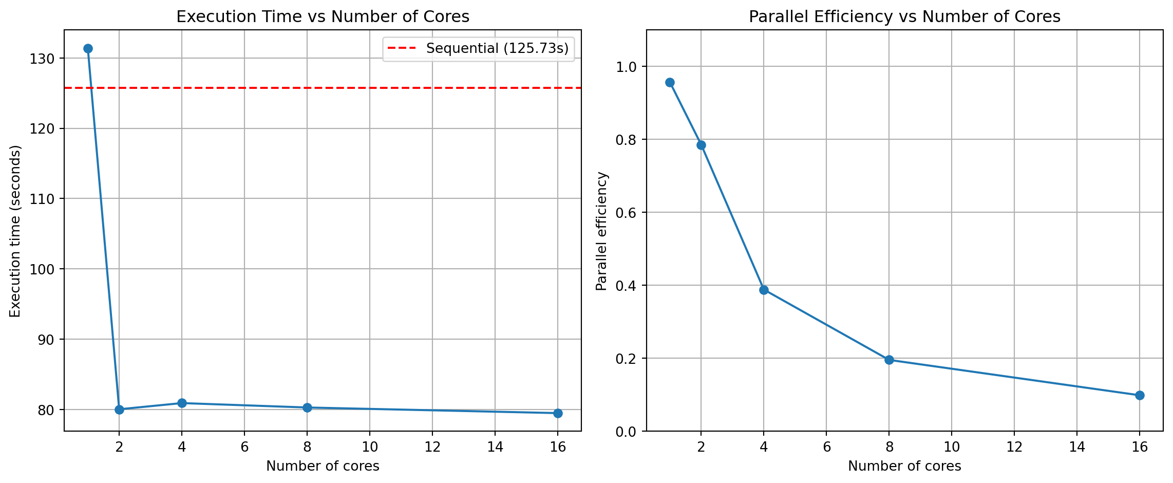
NoteOperating-system Differences in Parallelization Methods
Linux uses the fork method by default to start new processes, whereas macOS and Windows use the spawn method. This leads to differences in how processes are handled across operating systems. We use the functionality of set_all_seeds to ensure that the evaluation remains reproducible across all operating systems.