import numpy as np
import matplotlib.pyplot as plt
from spotpython.fun.objectivefunctions import Analytical
from spotpython.utils.init import fun_control_init, surrogate_control_init
from spotpython.spot import Spot23 User-Specified Functions: Extending the Analytical Class
This chapter illustrates how user-specified functions can be optimized and analyzed. It covers singe-objective function in Section 23.2 and multi-objective functions in Section 23.6, and how to use the spotpython package to optimize them. It shows a simple approach to define a user-specified function, both for single- and multi-objective optimization, and how to extend the Analytical class to create a custom function.
NoteCitation
- If this document has been useful to you and you wish to cite it in a scientific publication, please refer to the following paper, which can be found on arXiv: https://arxiv.org/abs/2307.10262.
@ARTICLE{bart23iArXiv,
      author = {{Bartz-Beielstein}, Thomas},
      title = "{Hyperparameter Tuning Cookbook:
          A guide for scikit-learn, PyTorch, river, and spotpython}",
     journal = {arXiv e-prints},
    keywords = {Computer Science - Machine Learning,
      Computer Science - Artificial Intelligence, 90C26, I.2.6, G.1.6},
         year = 2023,
        month = jul,
          eid = {arXiv:2307.10262},
          doi = {10.48550/arXiv.2307.10262},
archivePrefix = {arXiv},
       eprint = {2307.10262},
 primaryClass = {cs.LG}
}
23.1 Software Requirements
- The code examples in this chapter require the
spotpythonpackage, which can be installed viapip. - Furthermore, the following Python packages are required:
23.2 The Single-Objective Function: User Specified
We will use an analytical objective function, i.e., a function that can be described by a (closed) formula: \[ f(x) = \sum_i^k x_i^4. \]
This function is continuous, convex and unimodal. Since it returns one value for each input vector, it is a single-objective function. Multiple-objective functions can also be handled by spotpython. They are covered in Section 23.6.
The global minimum of the single-objective function is \[ f(x) = 0, \text{at } x = (0,0, \ldots, 0). \]
It can be implemented in Python as follows:
def user_fun(X):
    return(np.sum((X) **4, axis=1))
For example, if we have \(X = (1, 2, 3)\), then \[ f(x) = 1^4 + 2^4 + 3^4 = 1 + 16 + 81 = 98, \] and if we have \(X = (4, 5, 6)\), then \[ f(x) = 4^4 + 5^4 + 6^4 = 256 + 625 + 1296 = 2177. \]
We can pass a 2D array to the function, and it will return a 1D array with the results for each row:
user_fun(np.array([[1, 2, 3], [4, 5, 6]]))array([ 98, 2177])To make user_fun compatible with the spotpython package, we need to extend its argument list, so that it can handle the fun_control dictionary.
def user_fun(X, fun_control=None):
    return(np.sum((X) **4, axis=1))
Alternatively, you can add the **kwargs argument to the function, which will allow you to pass any additional keyword arguments:
def user_fun(X, **kwargs):
    return(np.sum((X) **4, axis=1))
fun_control = fun_control_init(
lower = np.array( [-1, -1]),
upper = np.array([1, 1]),
)
S = Spot(fun=user_fun,
fun_control=fun_control)
S.run()
S.plot_progress()spotpython tuning: 3.715394917589437e-05 [#######---] 73.33%. Success rate: 0.00%
spotpython tuning: 3.715394917589437e-05 [########--] 80.00%. Success rate: 0.00%
spotpython tuning: 3.715394917589437e-05 [#########-] 86.67%. Success rate: 0.00%
spotpython tuning: 3.715394917589437e-05 [#########-] 93.33%. Success rate: 0.00%
spotpython tuning: 3.715394917589437e-05 [##########] 100.00%. Success rate: 0.00% Done...
Experiment saved to 000_res.pkl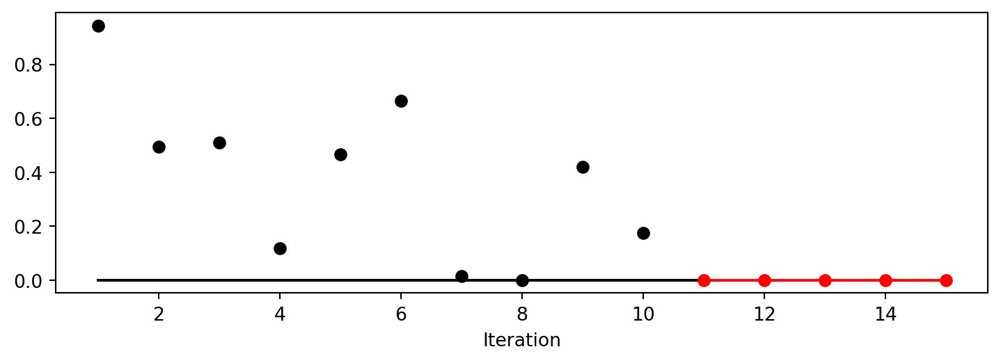
NoteSummary: Using
spotpython with Single-Objective User-Specified Functions
spotpythonaccepts user-specified functions that can be defined in Python.- The function should accept a 2D array as input and return a 1D array as output.
- The function can be defined with an additional argument
fun_controlto handle control parameters. - The
fun_controldictionary can be initialized with thefun_control_initfunction, which allows you to specify the bounds of the input variables.
23.3 The Objective Function: Extending the Analytical Class
- The
Analyticalclass is a base class for analytical functions in thespotpythonpackage. - It provides a framework for defining and evaluating analytical functions, including the ability to add noise to the output.
- The
Analyticalclass can be extended as follows:
from typing import Optional, Dict

class UserAnalytical(Analytical):
    def fun_user_function(self, X: np.ndarray, fun_control: Optional[Dict] = None) -> np.ndarray:
        """
        Custom new function: f(x) = x^4

        Args:
            X (np.ndarray): Input data as a 2D array.
            fun_control (Optional[Dict]): Control parameters for the function.

        Returns:
            np.ndarray: Computed values with optional noise.

        Examples:
            >>> import numpy as np
            >>> X = np.array([[1, 2, 3], [4, 5, 6]])
            >>> fun = UserAnalytical()
            >>> fun.fun_user_function(X)
        """
        X = self._prepare_input_data(X, fun_control)

        offset = np.ones(X.shape[1]) * self.offset
        y = np.sum((X - offset) **4, axis=1)

        # Add noise if specified in fun_control
return self._add_noise(y)- In comparison to the
user_funfunction, theUserAnalyticalclass provides additional functionality, such as adding noise to the output and preparing the input data. - First, we use the
user_funfunction as above.
user_fun = UserAnalytical()
X = np.array([[0, 0, 0], [1, 1, 1]])
results = user_fun.fun_user_function(X)
print(results)
[0. 3.]- Then we can add an offset to the function, which will shift the function by a constant value. This is useful for testing the optimization algorithm’s ability to find the global minimum.
user_fun = UserAnalytical(offset=1.0)
X = np.array([[0, 0, 0], [1, 1, 1]])
results = user_fun.fun_user_function(X)
print(results)
[3. 0.]- And, we can add noise to the function, which will add a random value to the output. This is useful for testing the optimization algorithm’s ability to find the global minimum in the presence of noise.
user_fun = UserAnalytical(sigma=1.0)
X = np.array([[0, 0, 0], [1, 1, 1]])
results = user_fun.fun_user_function(X)
print(results)
[0.06691138 3.11495313]- Here is an example of how to use the
UserAnalyticalclass with thespotpythonpackage:
user_fun = UserAnalytical().fun_user_function
fun_control = fun_control_init(
              PREFIX="USER",
              lower = -1.0*np.ones(2),
              upper = np.ones(2),
              var_name=["User Pressure", "User Temp"],
              TENSORBOARD_CLEAN=True,
              tensorboard_log=True)
spot_user = Spot(fun=user_fun,
                  fun_control=fun_control)
spot_user.run()
Moving TENSORBOARD_PATH: runs/ to TENSORBOARD_PATH_OLD: runs_OLD/runs_2025_11_06_17_23_40_0
Created spot_tensorboard_path: runs/spot_logs/USER_maans08_2025-11-06_17-23-40 for SummaryWriter()
spotpython tuning: 3.715394917589437e-05 [#######---] 73.33%. Success rate: 0.00%
spotpython tuning: 3.715394917589437e-05 [########--] 80.00%. Success rate: 0.00%
spotpython tuning: 3.715394917589437e-05 [#########-] 86.67%. Success rate: 0.00%
spotpython tuning: 3.715394917589437e-05 [#########-] 93.33%. Success rate: 0.00%
spotpython tuning: 3.715394917589437e-05 [##########] 100.00%. Success rate: 0.00% Done...
Experiment saved to USER_res.pkl<spotpython.spot.spot.Spot at 0x164ea3ed0>23.4 Results
_ = spot_user.print_results()min y: 3.715394917589437e-05
User Pressure: 0.05170658955305796
User Temp: 0.07401195908206382spot_user.plot_progress()
23.5 A Contour Plot
We can select two dimensions, say \(i=0\) and \(j=1\), and generate a contour plot as follows.
NoteNote:
We have specified identical min_z and max_z values to generate comparable plots.
spot_user.plot_contour(i=0, j=1, min_z=0, max_z=2.25)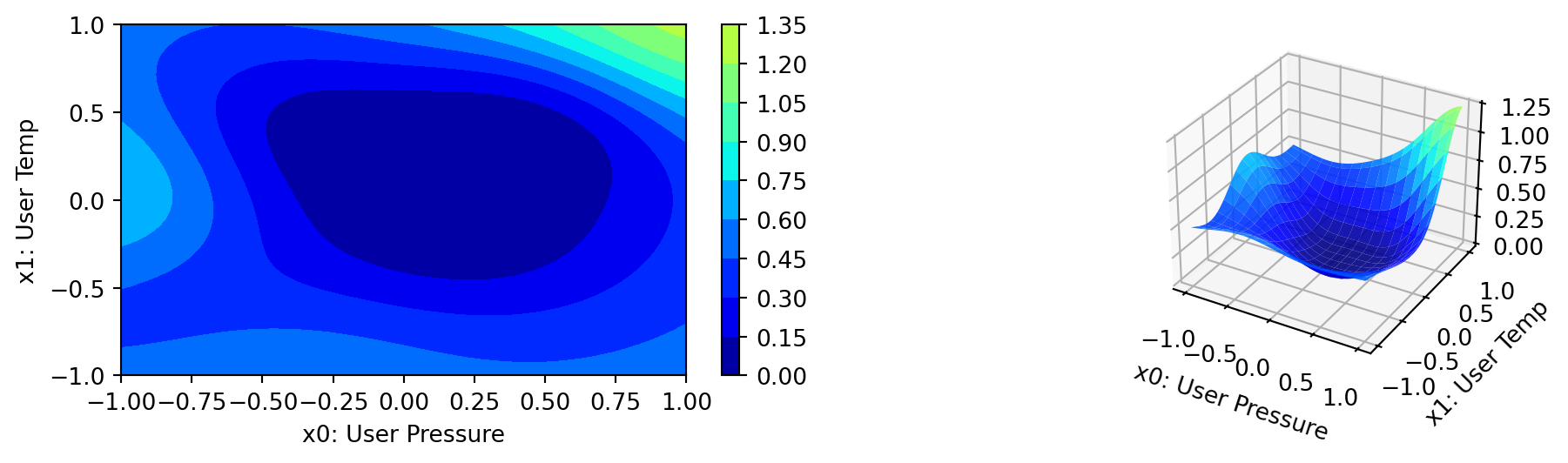
- The variable importance:
_ = spot_user.print_importance()User Pressure: 59.78437370790242
User Temp: 100.0spot_user.plot_importance()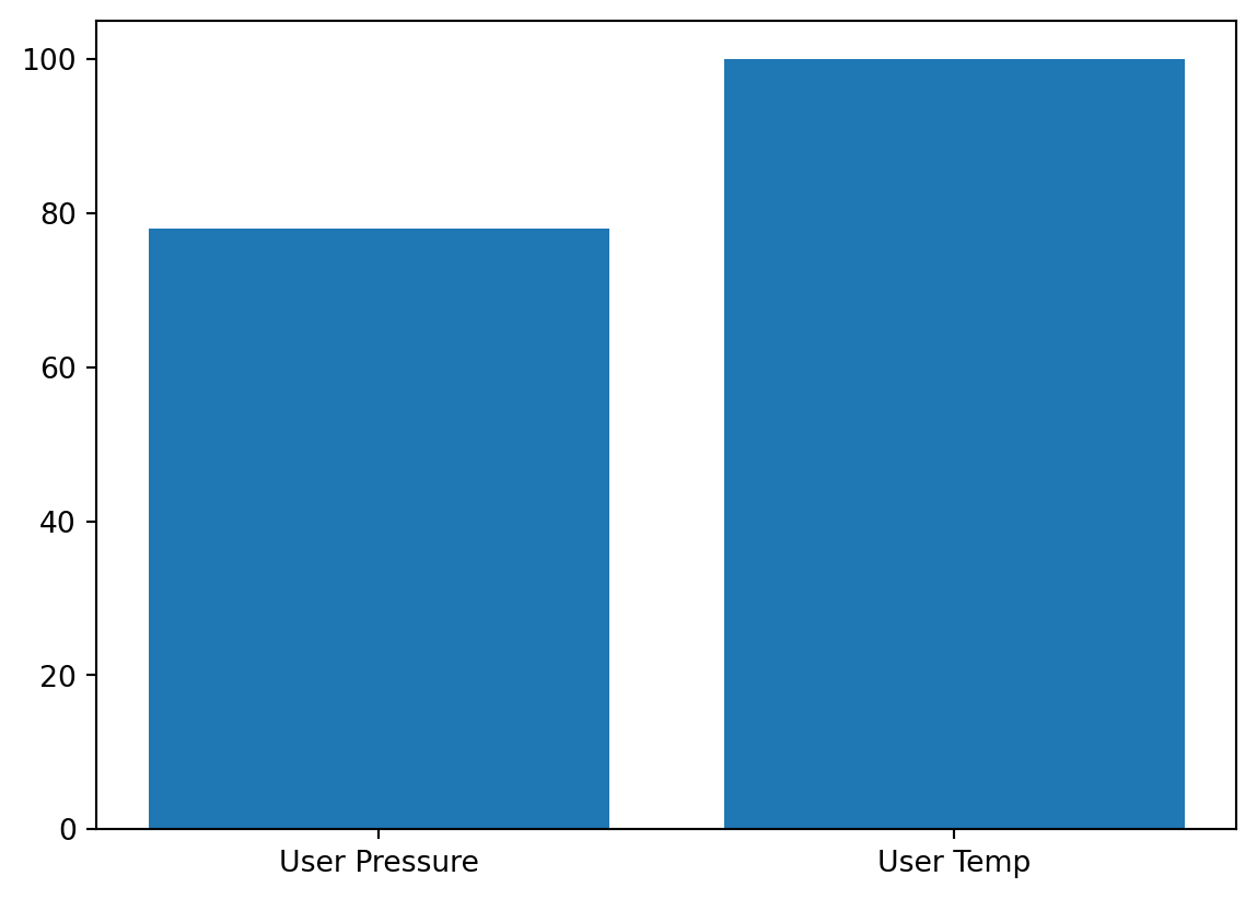
23.6 Multi-Objective Functions
- The
spotpythonpackage can also handle multi-objective functions, which are functions that return multiple values for each input vector. - As noted in Section 23.2, in the single-objective case, the function returns one value for each input vector and
spotpythonexpects a 1D array as output. - If the function returns a 2D array as output,
spotpythonwill treat it as a multi-objective function result.
23.6.1 Response Surface Experiment
Myers, Montgomery, and Anderson-Cook (2016) describe a response surface experiment where three input variables (reaction time, reaction temperature, and percent catalyst) were used to model two characteristics of a chemical reaction: percent conversion and thermal activity. Their model is based on the following equations:
\[\begin{align*} f_{\text{con}}(x) = & 81.09 + 1.0284 \cdot x_1 + 4.043 \cdot x_2 + 6.2037 \cdot x_3 + 1.8366 \cdot x_1^2 + 2.9382 \cdot x_2^2 \\ & + 5.1915 \cdot x_3^2 + 2.2150 \cdot x_1 \cdot x_2 + 11.375 \cdot x_1 \cdot x_3 + 3.875 \cdot x_2 \cdot x_3 \end{align*}\] and \[\begin{align*} f_{\text{act}}(x) = & 59.85 + 3.583 \cdot x_1 + 0.2546 \cdot x_2 + 2.2298 \cdot x_3 + 0.83479 \cdot x_1^2 + 0.07484 \cdot x_2^2 \\ & + 0.05716 \cdot x_3^2 + 0.3875 \cdot x_1 \cdot x_2 + 0.375 \cdot x_1 \cdot x_3 + 0.3125 \cdot x_2 \cdot x_3. \end{align*}\]
23.6.1.1 Defining the Multi-Objective Function myer16a
- The multi-objective function
myer16acombines the results of two single-objective functions: conversion and activity. - It is implemented in
spotpythonas follows:
import numpy as np

def conversion_pred(X):
    """
    Compute conversion predictions for each row in the input array.

    Args:
        X (np.ndarray): 2D array where each row is a configuration.

    Returns:
        np.ndarray: 1D array of conversion predictions.
    """
    return (
        81.09
        + 1.0284 * X[:, 0]
        + 4.043 * X[:, 1]
        + 6.2037 * X[:, 2]
        - 1.8366 * X[:, 0]**2
        + 2.9382 * X[:, 1]**2
        - 5.1915 * X[:, 2]**2
        + 2.2150 * X[:, 0] * X[:, 1]
        + 11.375 * X[:, 0] * X[:, 2]
        - 3.875 * X[:, 1] * X[:, 2]
    )

def activity_pred(X):
    """
    Compute activity predictions for each row in the input array.

    Args:
        X (np.ndarray): 2D array where each row is a configuration.

    Returns:
        np.ndarray: 1D array of activity predictions.
    """
    return (
        59.85
        + 3.583 * X[:, 0]
        + 0.2546 * X[:, 1]
        + 2.2298 * X[:, 2]
        + 0.83479 * X[:, 0]**2
        + 0.07484 * X[:, 1]**2
        + 0.05716 * X[:, 2]**2
        - 0.3875 * X[:, 0] * X[:, 1]
        - 0.375 * X[:, 0] * X[:, 2]
        + 0.3125 * X[:, 1] * X[:, 2]
    )

def fun_myer16a(X, fun_control=None):
    """
    Compute both conversion and activity predictions for each row in the input array.

    Args:
        X (np.ndarray): 2D array where each row is a configuration.
        fun_control (dict, optional): Additional control parameters (not used here).

    Returns:
        np.ndarray: 2D array where each row contains [conversion_pred, activity_pred].
    """
    return np.column_stack((conversion_pred(X), activity_pred(X)))
Now the function returns a 2D array with two columns, one for each objective function. The first column corresponds to the conversion prediction, and the second column corresponds to the activity prediction.
X = np.array([[1, 2, 3], [4, 5, 6]])
results = fun_myer16a(X)
print(results)
[[ 87.3132 72.25519]
[200.8662 98.7442 ]]23.6.1.2 Using a Weighted Sum
- The
spotpythonpackage can also handle multi-objective functions, which are functions that return multiple values for each input vector. - In this case, we can use a weighted sum to combine the two objectives into a single objective function.
- The function
aggergatetakes the two objectives and combines them into a single objective function by applying weights to each objective. - The weights can be adjusted to give more importance to one objective over the other.
- For example, if we want to give more importance to the conversion prediction, we can set the weight for the conversion prediction to 2 and the weight for the activity prediction to 0.1.
# Weight first objective with 2, second with 1/10
def aggregate(y):
    return np.sum(y*np.array([2, 0.1]), axis=1)
The aggregate function object is passed to the fun_control dictionary aas the fun_mo2so argument.
fun_control = fun_control_init(
              lower = np.array( [0, 0, 0]),
              upper = np.array([1, 1, 1]),
              fun_mo2so=aggregate)
S = Spot(fun=fun_myer16a,
        fun_control=fun_control)
S.run()
S.plot_progress()
spotpython tuning: 168.41794461566062 [#######---] 73.33%. Success rate: 100.00%
spotpython tuning: 168.35654210764483 [########--] 80.00%. Success rate: 100.00%
spotpython tuning: 168.16500000000002 [#########-] 86.67%. Success rate: 100.00%
Using spacefilling design as fallback.
spotpython tuning: 168.16500000000002 [#########-] 93.33%. Success rate: 75.00%
spotpython tuning: 166.99037900000002 [##########] 100.00%. Success rate: 80.00% Done...
Experiment saved to 000_res.pkl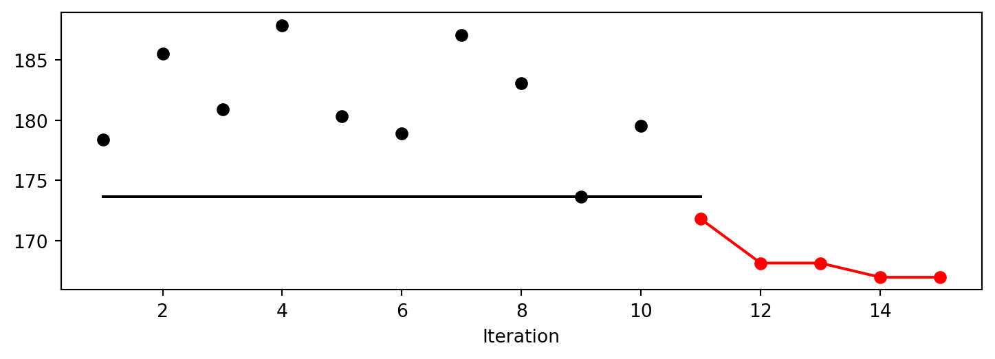
If no fun_mo2so function is specified, the spotpython package will use the first return value of the multi-objective function as the single objective function.
spotpython allows access to the complete history of multi-objective return values. They are stored in the y_mo attribute of the Spot object. The y_mo attribute is a 2D array where each row corresponds to a configuration and each column corresponds to an objective function. These values can be visualized as shown in Figure 23.1.
y_mo = S.y_mo
y = S.y
plt.xlim(0, len(y_mo))
plt.ylim(0.9 * np.min(y_mo), 1.1* np.max(y))
plt.scatter(range(len(y_mo)), y_mo[:, 0], label='Conversion', marker='o')
plt.scatter(range(len(y_mo)), y_mo[:, 1], label='Activity', marker='x')
plt.plot(np.minimum.accumulate(y_mo[:, 0]), label='Cum. Min Conversion')
plt.plot(np.minimum.accumulate(y_mo[:, 1]), label='Cum. Min Activity')
plt.scatter(range(len(y)), y, label='Agg. Result', marker='D', color='red')
plt.plot(np.minimum.accumulate(y), label='Cum. Min Agg. Res.', color='red')
plt.xlabel('Iteration')
plt.ylabel('Objective Function Value')
plt.grid()
plt.title('Single- and Multi-Obj. Function Values')
plt.legend(loc='upper left', bbox_to_anchor=(1, 1))
plt.tight_layout()
plt.show()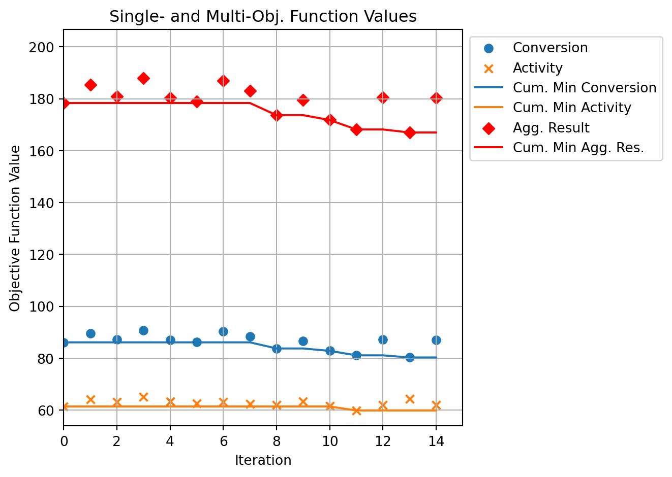
Since all values from the multi-objective functions can be accessed, more sophisticated multi-objective optimization methods can be implemented. For example, the spotpython package provides a pareto_front function that can be used to compute the Pareto front of the multi-objective function values, see pareto. The Pareto front is a set of solutions that are not dominated by any other solution in the objective space.
NoteSummary: Using
spotpython with Multi-Objective User-Specified Functions
spotpythonaccepts user-specified multi-objective functions that can be defined in Python.- The function should accept a 2D array as input and return a 2D array as output.
- An
aggregatefunction can be used to combine multiple objectives into a single objective function.
23.7 Jupyter Notebook
Note
- The Jupyter-Notebook of this lecture is available on GitHub in the Hyperparameter-Tuning-Cookbook Repository