from spotpython.design.spacefilling import SpaceFilling
from spotpython.surrogate.kriging import Kriging
from spotpython.fun.objectivefunctions import Analytical
import numpy as np22 Factorial Variables
Until now, we have considered continuous variables. However, in many applications, the variables are not continuous, but rather discrete or categorical. For example, the number of layers in a neural network, the number of trees in a random forest, or the type of kernel in a support vector machine are all discrete variables. In the following, we will consider a simple example with two numerical variables and one categorical variable.
First, we generate the test data set for fitting the Kriging model. We use the SpaceFilling class to generate the first two diemnsion of \(n=30\) design points. The third dimension is a categorical variable, which can take the values \(0\), \(1\), or \(2\).
gen = SpaceFilling(2)
n = 30
rng = np.random.RandomState(1)
lower = np.array([-5,-0])
upper = np.array([10,15])
fun_orig = Analytical().fun_branin
fun = Analytical().fun_branin_factor

X0 = gen.scipy_lhd(n, lower=lower, upper = upper)
X1 = np.random.randint(low=0, high=3, size=(n,))
X = np.c_[X0, X1]
print(X[:5,:])
[[-2.84117593 5.97308949 1. ]
[-3.61017994 6.90781409 1. ]
[ 9.91204705 5.09395275 1. ]
[-4.4616725 1.3617128 1. ]
[-2.40987728 8.05505365 1. ]]The objective function is the fun_branin_factor in the analytical class [SOURCE]. It calculates the Branin function of \((x_1, x_2)\) with an additional factor based on the value of \(x_3\). If \(x_3 = 1\), the value of the Branin function is increased by 10. If \(x_3 = 2\), the value of the Branin function is decreased by 10. Otherwise, the value of the Branin function is not changed.
y = fun(X)
y_orig = fun_orig(X0)
data = np.c_[X, y_orig, y]
print(data[:5,:])
[[ -2.84117593 5.97308949 1. 32.09388125 42.09388125]
[ -3.61017994 6.90781409 1. 43.965223 53.965223 ]
[ 9.91204705 5.09395275 1. 6.25588575 16.25588575]
[ -4.4616725 1.3617128 1. 212.41884106 222.41884106]
[ -2.40987728 8.05505365 1. 9.25981051 19.25981051]]We fit two Kriging models, one with three numerical variables and one with two numerical variables and one categorical variable. We then compare the predictions of the two models.
S = Kriging(name='kriging',  seed=123, log_level=50, method="interpolation", var_type=["num", "num", "num"])
S.fit(X, y)
Sf = Kriging(name='kriging',  seed=123, log_level=50, method="interpolation", var_type=["num", "num", "factor"])
Sf.fit(X, y)
Kriging(eps=np.float64(1.4901161193847656e-08), kernel_params={},
method='interpolation', model_fun_evals=100,
model_optimizer=<function differential_evolution at 0x11009a3e0>,
n_theta=3, name='kriging', seed=123,
theta=array([-1.62828409, -3. , -3. ]),
var_type=['num', 'num', 'factor'])In a Jupyter environment, please rerun this cell to show the HTML representation or trust the notebook. On GitHub, the HTML representation is unable to render, please try loading this page with nbviewer.org.
Parameters
| eps | np.float64(1....193847656e-08) | |
| penalty | 10000.0 | |
| method | 'interpolation' | |
| var_type | ['num', 'num', ...] | |
| name | 'kriging' | |
| seed | 123 | |
| model_optimizer | <function dif...t 0x11009a3e0> | |
| model_fun_evals | 100 | |
| n_theta | 3 | |
| min_theta | -3.0 | |
| max_theta | 2.0 | |
| theta_init_zero | False | |
| p_val | 2.0 | |
| n_p | 1 | |
| optim_p | False | |
| min_p | 1.0 | |
| max_p | 2.0 | |
| min_Lambda | -9.0 | |
| max_Lambda | 0.0 | |
| log_level | 50 | |
| spot_writer | None | |
| counter | None | |
| metric_factorial | 'canberra' | |
| isotropic | False | |
| theta | array([-1.628... -3. ]) | |
| Lambda | None | |
| use_nystrom | False | |
| nystrom_m | None | |
| nystrom_seed | 1234 | |
| kernel | 'gauss' | |
| kernel_params | {} |
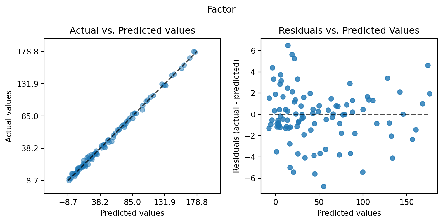
We can now compare the predictions of the two models. We generate a new test data set and calculate the sum of the absolute differences between the predictions of the two models and the true values of the objective function. If the categorical variable is important, the sum of the absolute differences should be smaller than if the categorical variable is not important.
n = 100
k = 100
y_true = np.zeros(n*k)
y_pred= np.zeros(n*k)
y_factor_pred= np.zeros(n*k)
for i in range(k):
  X0 = gen.scipy_lhd(n, lower=lower, upper = upper)
  X1 = np.random.randint(low=0, high=3, size=(n,))
  X = np.c_[X0, X1]
  a = i*n
  b = (i+1)*n
  y_true[a:b] = fun(X)
  y_pred[a:b] = S.predict(X)
  y_factor_pred[a:b] = Sf.predict(X)
import pandas as pd
df = pd.DataFrame({"y":y_true, "Prediction":y_pred, "Prediction_factor":y_factor_pred})
df.head()| y | Prediction | Prediction_factor | |
|---|---|---|---|
| 0 | -3.315251 | 12.360036 | 3.614671 |
| 1 | 95.865258 | 95.909885 | 95.826516 |
| 2 | 39.811774 | 44.983563 | 40.151519 |
| 3 | 8.177150 | 18.245032 | 7.238393 |
| 4 | 10.968377 | 10.026556 | 3.459984 |
df.tail()| y | Prediction | Prediction_factor | |
|---|---|---|---|
| 9995 | 73.620503 | 74.028282 | 74.431207 |
| 9996 | 76.187178 | 80.840493 | 79.482086 |
| 9997 | 39.494401 | 48.040580 | 39.543576 |
| 9998 | 15.390268 | 4.594148 | 17.076011 |
| 9999 | 26.261264 | 29.681827 | 26.539651 |
s=np.sum(np.abs(y_pred - y_true))
sf=np.sum(np.abs(y_factor_pred - y_true))
res = (sf - s)
print(res)-22717.936175748313from spotpython.plot.validation import plot_actual_vs_predicted
plot_actual_vs_predicted(y_test=df["y"], y_pred=df["Prediction"], title="Default")
plot_actual_vs_predicted(y_test=df["y"], y_pred=df["Prediction_factor"], title="Factor")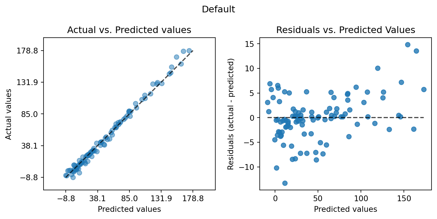
22.1 Jupyter Notebook
Note
- The Jupyter-Notebook of this lecture is available on GitHub in the Hyperparameter-Tuning-Cookbook Repository