import numpy as np
from spotpython.fun.objectivefunctions import Analytical
from spotpython.utils.init import fun_control_init, surrogate_control_init, design_control_init
from spotpython.spot import Spot13 Multi-dimensional Functions
This chapter illustrates how high-dimensional functions can be optimized and analyzed. For reasons of illustration, we will use the three-dimensional Sphere function, which is a simple and well-known function. The problem dimension is \(k=3\), but can be easily adapted to other, higher dimensions.
13.1 The Objective Function: 3-dim Sphere
The spotpython package provides several classes of objective functions. We will use an analytical objective function, i.e., a function that can be described by a (closed) formula: \[
f(x) = \sum_i^k x_i^2.
\]
The Sphere function is continuous, convex and unimodal. The plot shows its two-dimensional form. The global minimum is \[ f(x) = 0, \text{at } x = (0,0, \ldots, 0). \]
It is available as fun_sphere in the Analytical class [SOURCE].
fun = Analytical().fun_sphereHere we will use problem dimension \(k=3\), which can be specified by the lower bound arrays. The size of the lower bound array determines the problem dimension. If we select -1.0 * np.ones(3), a three-dimensional function is created.
In contrast to the one-dimensional case (Section 12.25), where only one theta value was used, we will use three different theta values (one for each dimension). This is done automatically, because the setting isotropic=False is the default in the surrogate_control. As default, spotpython uses separate theta values for each problem dimension. More specifically, if isotropic is set to True, only one theta value is used for all dimensions. If isotropic is set to False, then the \(k\) theta values are used, where \(k\) is the problem dimension. The meaning of “isotropic” is explained in @#sec-iso-aniso-kriging.
The prefix is set to "03" to distinguish the results from the one-dimensional case. Again, TensorBoard can be used to monitor the progress of the optimization.
We can also add interpretable labels to the dimensions, which will be used in the plots. Therefore, we set var_name=["Pressure", "Temp", "Lambda"] instead of the default var_name=None, which would result in the labels x_0, x_1, and x_2.
fun_control = fun_control_init(
              PREFIX="03",
              lower = -1.0*np.ones(3),
              upper = np.ones(3),
              var_name=["Pressure", "Temp", "Lambda"],
              TENSORBOARD_CLEAN=True,
              tensorboard_log=True)
surrogate_control = surrogate_control_init()
spot_3 = Spot(fun=fun,
                  fun_control=fun_control,
                  surrogate_control=surrogate_control)
spot_3.run()
Moving TENSORBOARD_PATH: runs/ to TENSORBOARD_PATH_OLD: runs_OLD/runs_2025_11_06_17_16_25_0
Created spot_tensorboard_path: runs/spot_logs/03_maans08_2025-11-06_17-16-25 for SummaryWriter()
spotpython tuning: 0.03443805738918038 [#######---] 73.33%. Success rate: 100.00%
spotpython tuning: 0.03134407473407909 [########--] 80.00%. Success rate: 100.00%
spotpython tuning: 0.0009627751650306065 [#########-] 86.67%. Success rate: 100.00%
spotpython tuning: 8.337474234130422e-05 [#########-] 93.33%. Success rate: 100.00%
spotpython tuning: 3.8172596925679106e-05 [##########] 100.00%. Success rate: 100.00% Done...
Experiment saved to 03_res.pkl<spotpython.spot.spot.Spot at 0x1049d3e00>
Note
Now we can start TensorBoard in the background with the following command:
tensorboard --logdir="./runs"and can access the TensorBoard web server with the following URL:
http://localhost:6006/13.1.1 Results
13.1.1.1 Best Objective Function Values
The best objective function value and its corresponding input values are printed as follows:
_ = spot_3.print_results()min y: 3.8172596925679106e-05
Pressure: 0.0036952312636787847
Temp: 0.0009377053161100289
Lambda: 0.004861951416226718The method plot_progress() plots current and best found solutions versus the number of iterations as shown in Figure 13.1.
spot_3.plot_progress()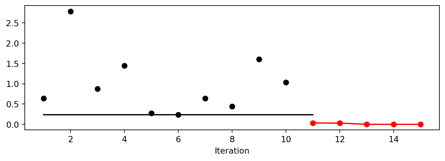
13.1.1.2 A Contour Plot
We can select two dimensions, say \(i=0\) and \(j=1\), and generate a contour plot as follows. Note, we have specified identical min_z and max_z values to generate comparable plots.
spot_3.plot_contour(i=0, j=1, min_z=0, max_z=2.25)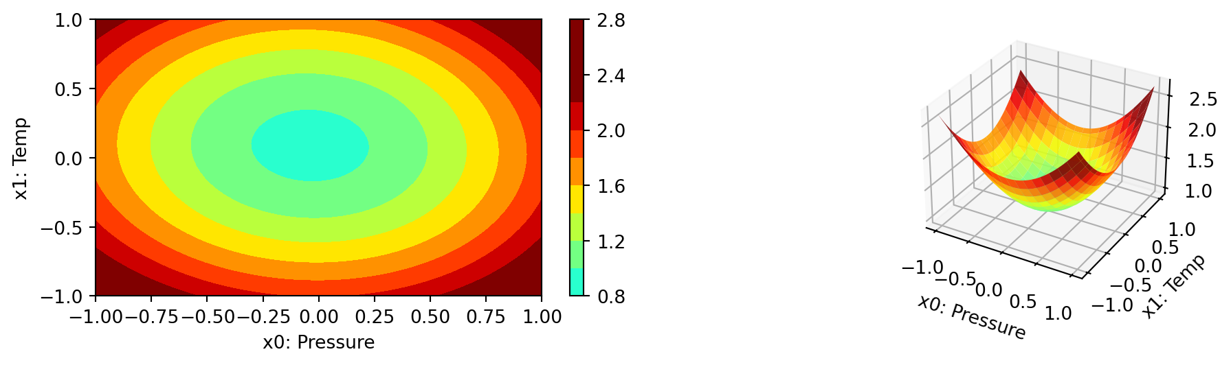
- In a similar manner, we can plot dimension \(i=0\) and \(j=2\):
spot_3.plot_contour(i=0, j=2, min_z=0, max_z=2.25)
- The final combination is \(i=1\) and \(j=2\):
spot_3.plot_contour(i=1, j=2, min_z=0, max_z=2.25)
- The three plots look very similar, because the
fun_sphereis symmetric. - This can also be seen from the variable importance:
_ = spot_3.print_importance()Pressure: 99.99999999999999
Temp: 99.17928367751998
Lambda: 91.43655243996746spot_3.plot_importance()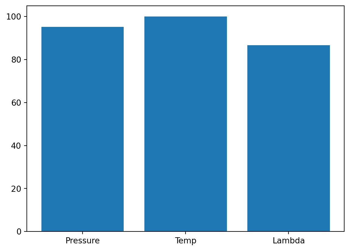
13.1.2 TensorBoard
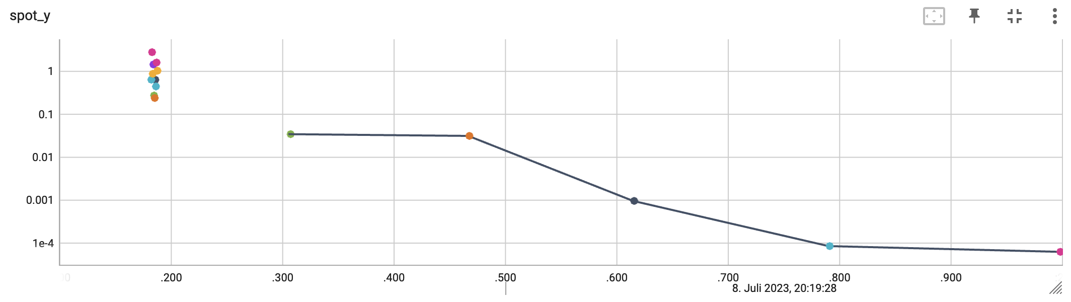
The second TensorBoard visualization shows the input values, i.e., \(x_0, \ldots, x_2\), plotted against the wall time. 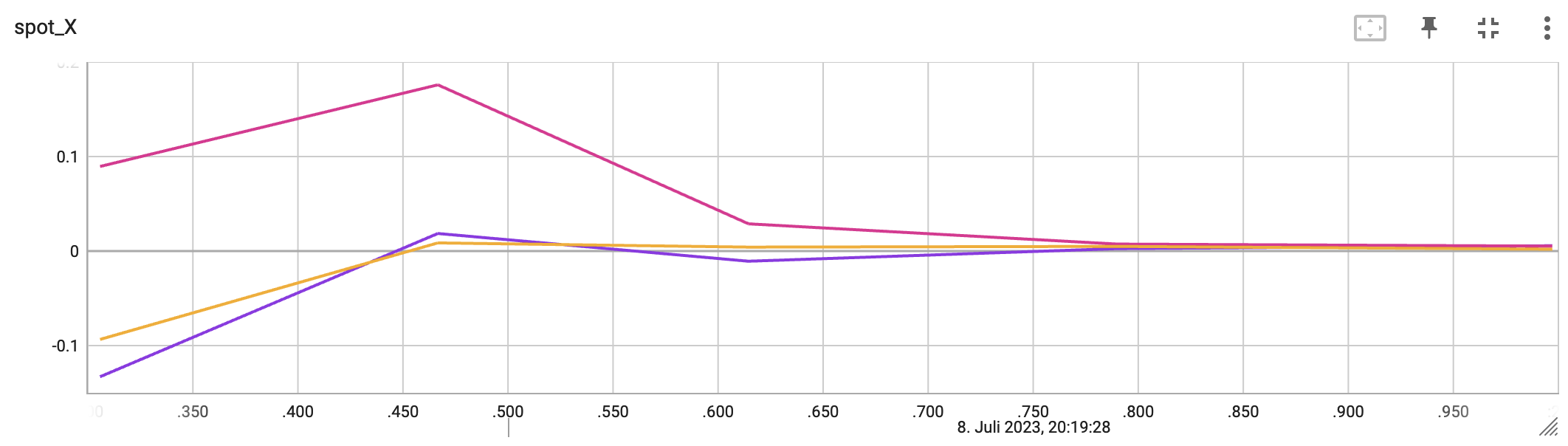
The third TensorBoard plot illustrates how spotpython can be used as a microscope for the internal mechanisms of the surrogate-based optimization process. Here, one important parameter, the learning rate \(\theta\) of the Kriging surrogate is plotted against the number of optimization steps.

13.1.3 Conclusion
Based on this quick analysis, we can conclude that all three dimensions are equally important (as expected, because the Analytical function is known).
13.2 Exercises
Exercise 13.1 (The Three Dimensional fun_cubed) The spotpython package provides several classes of objective functions.
We will use the fun_cubed in the Analytical class [SOURCE]. The input dimension is 3. The search range is \(-1 \leq x \leq 1\) for all dimensions.
Tasks: * Generate contour plots * Calculate the variable importance. * Discuss the variable importance: * Are all variables equally important? * If not: * Which is the most important variable? * Which is the least important variable?
Exercise 13.2 (The Ten Dimensional fun_wing_wt)
- The input dimension is
10. The search range is \(0 \leq x \leq 1\) for all dimensions. - Calculate the variable importance.
- Discuss the variable importance:
- Are all variables equally important?
- If not:
- Which is the most important variable?
- Which is the least important variable?
- Generate contour plots for the three most important variables. Do they confirm your selection?
Exercise 13.3 (The Three Dimensional fun_runge)
- The input dimension is
3. The search range is \(-5 \leq x \leq 5\) for all dimensions. - Generate contour plots
- Calculate the variable importance.
- Discuss the variable importance:
- Are all variables equally important?
- If not:
- Which is the most important variable?
- Which is the least important variable?
Exercise 13.4 (The Three Dimensional fun_linear)
- The input dimension is
3. The search range is \(-5 \leq x \leq 5\) for all dimensions. - Generate contour plots
- Calculate the variable importance.
- Discuss the variable importance:
- Are all variables equally important?
- If not:
- Which is the most important variable?
- Which is the least important variable?
Exercise 13.5 (The Two Dimensional Rosenbrock Function fun_rosen)
- The input dimension is
2. The search range is \(-5 \leq x \leq 10\) for all dimensions. - See Rosenbrock function and Rosenbrock Function for details.
- Generate contour plots
- Calculate the variable importance.
- Discuss the variable importance:
- Are all variables equally important?
- If not:
- Which is the most important variable?
- Which is the least important variable?
13.3 Selected Solutions
Solution 13.1 (Solution to Exercise 13.1: The Three-dimensional Cubed Function fun_cubed). We instanciate the fun_cubed function from the Analytical class.
from spotpython.fun.objectivefunctions import Analytical
fun_cubed = Analytical().fun_cubed- Here we will use problem dimension \(k=3\), which can be specified by the
lowerbound arrays. The size of thelowerbound array determines the problem dimension. If we select-1.0 * np.ones(3), a three-dimensional function is created. - In contrast to the one-dimensional case, where only one
thetavalue was used, we will use three differentthetavalues (one for each dimension). - The prefix is set to
"03"to distinguish the results from the one-dimensional case. - We will set the
fun_evals=20to limit the number of function evaluations to 20 for this example. - The size of the initial design is set to
10by default. It can be changed by settinginit_size=10viadesign_control_initin thedesign_controldictionary. - Again, TensorBoard can be used to monitor the progress of the optimization.
- We can also add interpretable labels to the dimensions, which will be used in the plots. Therefore, we set
var_name=["Pressure", "Temp", "Lambda"]instead of the defaultvar_name=None, which would result in the labelsx_0,x_1, andx_2.
Here is the link to the documentation of the fun_control_init function: [DOC]. The documentation of the design_control_init function can be found here: [DOC].
The setup can be done as follows:
fun_control = fun_control_init(
              PREFIX="cubed",
              fun_evals=20,
              lower = -1.0*np.ones(3),
              upper = np.ones(3),
              var_name=["Pressure", "Temp", "Lambda"],
              TENSORBOARD_CLEAN=True,
              tensorboard_log=True
              )

surrogate_control = surrogate_control_init()
design_control = design_control_init(init_size=10)
Moving TENSORBOARD_PATH: runs/ to TENSORBOARD_PATH_OLD: runs_OLD/runs_2025_11_06_17_16_30_0
Created spot_tensorboard_path: runs/spot_logs/cubed_maans08_2025-11-06_17-16-30 for SummaryWriter()- After the setup, we can pass the dictionaries to the
Spotclass and run the optimization process.
spot_cubed = Spot(fun=fun_cubed,
                  fun_control=fun_control,
                  surrogate_control=surrogate_control)
spot_cubed.run()
spotpython tuning: -1.4616828410586926 [######----] 55.00%. Success rate: 100.00%
spotpython tuning: -1.4616828410586926 [######----] 60.00%. Success rate: 50.00%
spotpython tuning: -2.0973782471243143 [######----] 65.00%. Success rate: 66.67%
spotpython tuning: -2.0973782471243143 [#######---] 70.00%. Success rate: 50.00%
spotpython tuning: -2.0973782471243143 [########--] 75.00%. Success rate: 40.00%
spotpython tuning: -2.122182907736537 [########--] 80.00%. Success rate: 50.00%
spotpython tuning: -3.0 [########--] 85.00%. Success rate: 57.14%
Using spacefilling design as fallback.
spotpython tuning: -3.0 [#########-] 90.00%. Success rate: 50.00%
Using spacefilling design as fallback.
spotpython tuning: -3.0 [##########] 95.00%. Success rate: 44.44%
spotpython tuning: -3.0 [##########] 100.00%. Success rate: 40.00% Done...
Experiment saved to cubed_res.pkl<spotpython.spot.spot.Spot at 0x1565691d0>- Results
_ = spot_cubed.print_results()min y: -3.0
Pressure: -1.0
Temp: -1.0
Lambda: -1.0spot_cubed.plot_progress()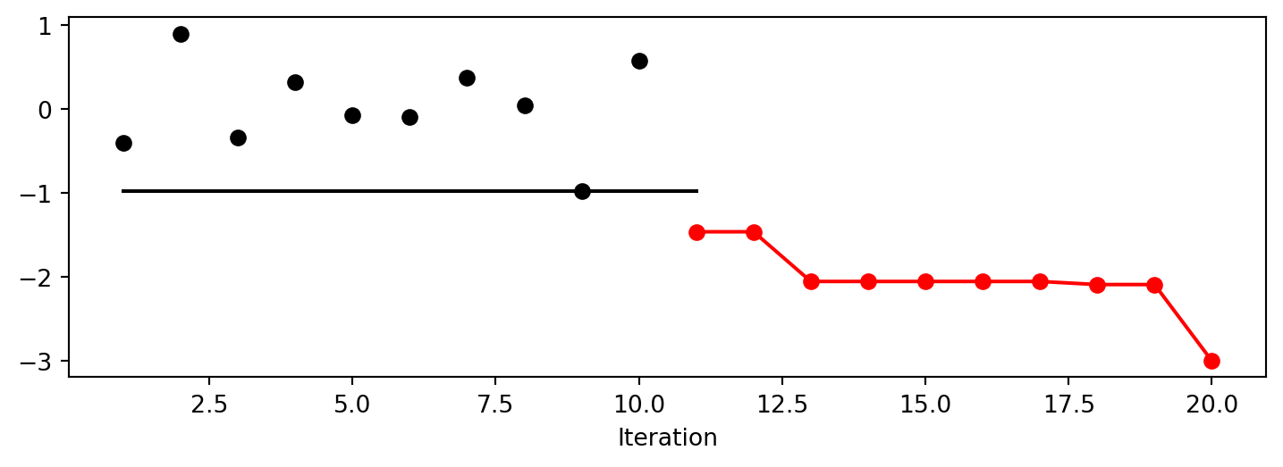
- Contour Plots
We can select two dimensions, say \(i=0\) and \(j=1\), and generate a contour plot as follows.
We can specify identical min_z and max_z values to generate comparable plots. The default values are min_z=None and max_z=None, which will be replaced by the minimum and maximum values of the objective function.
min_z = -3
max_z = 1
spot_cubed.plot_contour(i=0, j=1, min_z=min_z, max_z=max_z)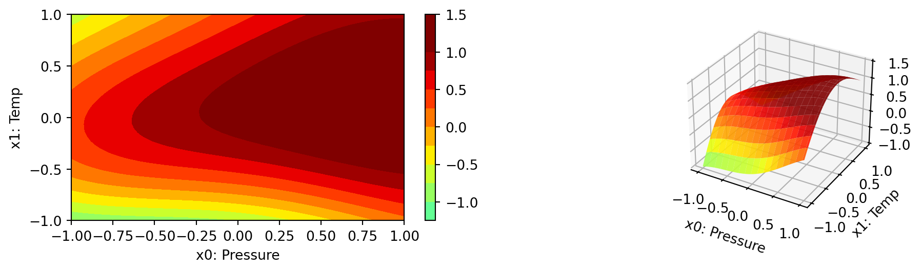
- In a similar manner, we can plot dimension \(i=0\) and \(j=2\):
spot_cubed.plot_contour(i=0, j=2, min_z=min_z, max_z=max_z)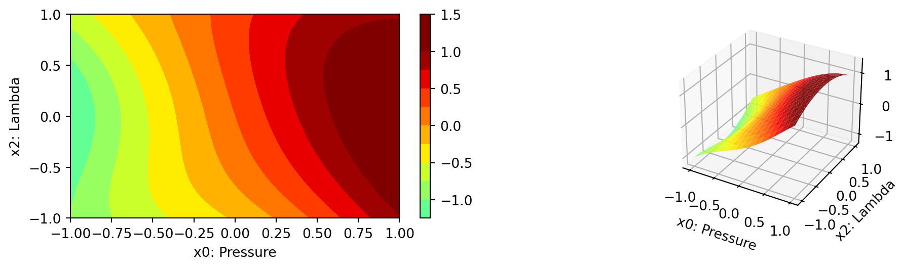
- The final combination is \(i=1\) and \(j=2\):
spot_cubed.plot_contour(i=1, j=2, min_z=min_z, max_z=max_z)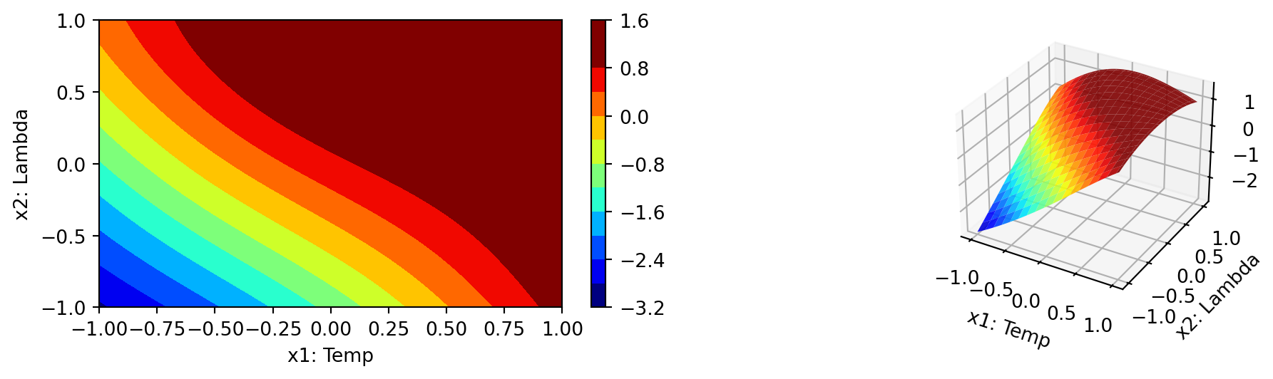
- The variable importance can be printed and visualized as follows:
_ = spot_cubed.print_importance()Pressure: 30.019890618668967
Temp: 100.0
Lambda: 93.41582927565221spot_cubed.plot_importance()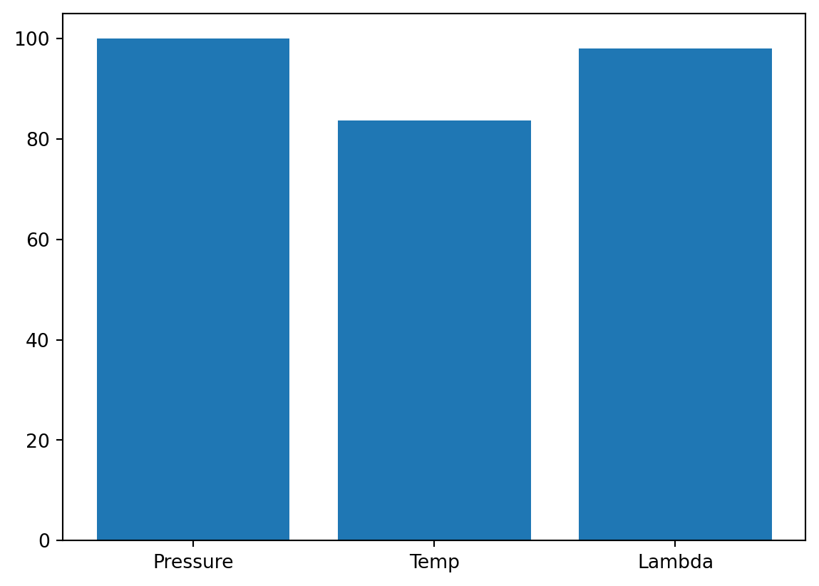
Solution 13.2 (Solution to Exercise 13.5: The Two-dimensional Rosenbrock Function fun_rosen).
import numpy as np
from spotpython.fun.objectivefunctions import Analytical
from spotpython.utils.init import fun_control_init, surrogate_control_init
from spotpython.spot import Spot- The Objective Function: 2-dim
fun_rosen
The spotpython package provides several classes of objective functions. We will use the fun_rosen in the Analytical class [SOURCE].
fun_rosen = Analytical().fun_rosen- Here we will use problem dimension \(k=2\), which can be specified by the
lowerbound arrays. - The size of the
lowerbound array determines the problem dimension. If we select-5.0 * np.ones(2), a two-dimensional function is created. - In contrast to the one-dimensional case, where only one
thetavalue is used, we will use \(k\) differentthetavalues (one for each dimension). - The prefix is set to
"ROSEN". - Again, TensorBoard can be used to monitor the progress of the optimization.
fun_control = fun_control_init(
              PREFIX="ROSEN",
              lower = -5.0*np.ones(2),
              upper = 10*np.ones(2),
              fun_evals=25)
surrogate_control = surrogate_control_init()
spot_rosen = Spot(fun=fun_rosen,
                  fun_control=fun_control,
                  surrogate_control=surrogate_control)
spot_rosen.run()
spotpython tuning: 90.77788110350957 [####------] 44.00%. Success rate: 100.00%
spotpython tuning: 1.0173064877521703 [#####-----] 48.00%. Success rate: 100.00%
spotpython tuning: 1.0173064877521703 [#####-----] 52.00%. Success rate: 66.67%
spotpython tuning: 1.0173064877521703 [######----] 56.00%. Success rate: 50.00%
spotpython tuning: 0.7867277329036355 [######----] 60.00%. Success rate: 60.00%
spotpython tuning: 0.7867277329036355 [######----] 64.00%. Success rate: 50.00%
spotpython tuning: 0.7867277329036355 [#######---] 68.00%. Success rate: 42.86%
spotpython tuning: 0.7867277329036355 [#######---] 72.00%. Success rate: 37.50%
spotpython tuning: 0.7867277329036355 [########--] 76.00%. Success rate: 33.33%
spotpython tuning: 0.7867277329036355 [########--] 80.00%. Success rate: 30.00%
spotpython tuning: 0.7867277329036355 [########--] 84.00%. Success rate: 27.27%
spotpython tuning: 0.7867277329036355 [#########-] 88.00%. Success rate: 25.00%
spotpython tuning: 0.7867277329036355 [#########-] 92.00%. Success rate: 23.08%
spotpython tuning: 0.7867277329036355 [##########] 96.00%. Success rate: 21.43%
spotpython tuning: 0.7867277329036355 [##########] 100.00%. Success rate: 20.00% Done...
Experiment saved to ROSEN_res.pkl<spotpython.spot.spot.Spot at 0x157abb750>Now we can start TensorBoard in the background with the following command:
tensorboard --logdir="./runs"and can access the TensorBoard web server with the following URL:
http://localhost:6006/- Results
_ = spot_rosen.print_results()min y: 0.7867277329036355
x0: 0.13953655588708272
x1: 0.08753688433642533spot_rosen.plot_progress(log_y=True)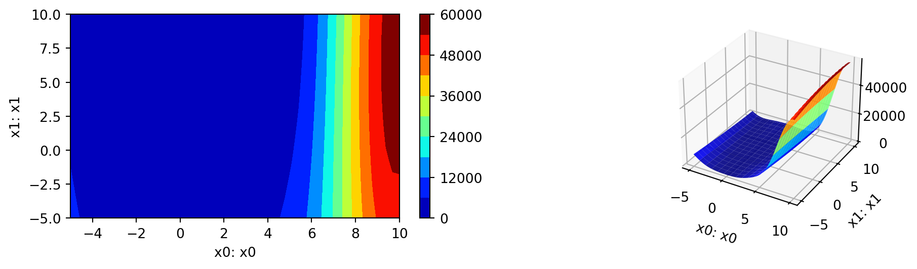
- A Contour Plot: We can select two dimensions, say \(i=0\) and \(j=1\), and generate a contour plot as follows.
- Note: For higher dimensions, it might be useful to have identical
min_zandmax_zvalues to generate comparable plots. The default values aremin_z=Noneandmax_z=None, which will be replaced by the minimum and maximum values of the objective function.
min_z = None
max_z = None
spot_rosen.plot_contour(i=0, j=1, min_z=min_z, max_z=max_z)
- The variable importance can be calculated as follows:
_ = spot_rosen.print_importance()x0: 99.99999999999999
x1: 2.2596151128068156spot_rosen.plot_importance()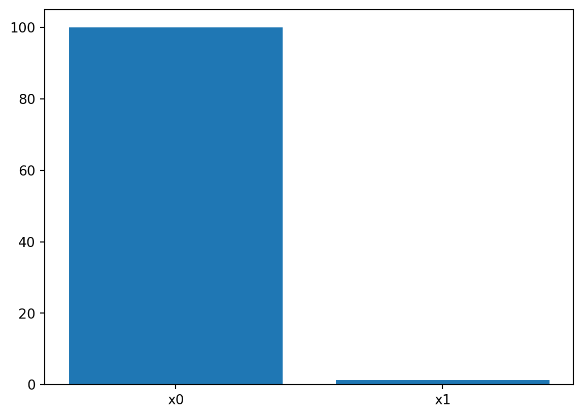
13.4 Jupyter Notebook
Note
- The Jupyter-Notebook of this lecture is available on GitHub in the Hyperparameter-Tuning-Cookbook Repository