Appendix E — Datasets

E.1 The Diabetes Data Set

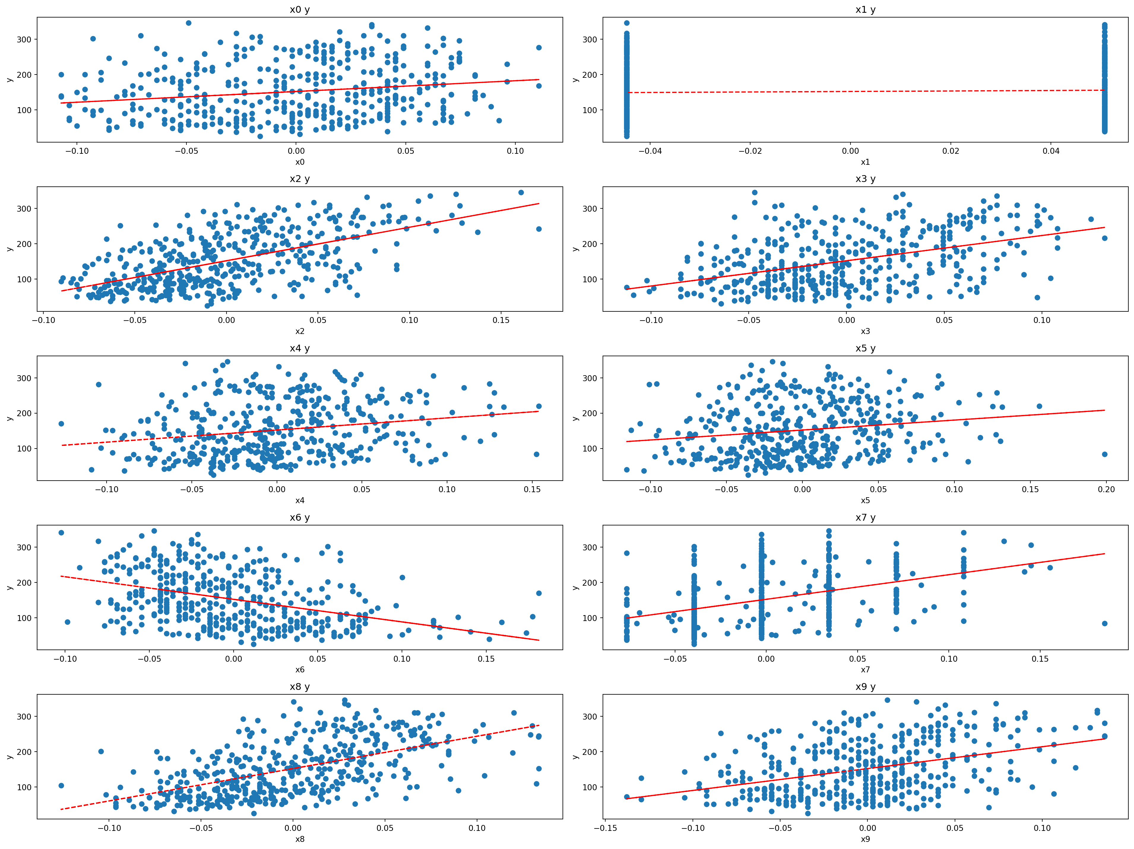
This section describes the Diabetes data set. This is a PyTorch Dataset for regression, which is derived from the Diabetes data set from scikit-learn (sklearn). Ten baseline variables, age, sex, body mass index, average blood pressure, and six blood serum measurements were obtained for each of n = 442 diabetes patients, as well as the response of interest, a quantitative measure of disease progression one year after baseline.

E.1.1 Data Exploration of the sklearn Diabetes Data Set

from sklearn.datasets import load_diabetes
from spotpython.plot.xy import plot_y_vs_X
data = load_diabetes()
X, y = data.data, data.target
plot_y_vs_X(X, y, nrows=5, ncols=2, figsize=(20, 15))

• Each of these 10 feature variables have been mean centered and scaled by the standard deviation times the square root of n_samples (i.e., the sum of squares of each column totals 1).

• s3_hdl shows a different behavior than the other features. It has a negative slope. HDL (high-density lipoprotein) cholesterol, sometimes called “good” cholesterol, absorbs cholesterol in the blood and carries it back to the liver. The liver then flushes it from the body. High levels of HDL cholesterol can lower your risk for heart disease and stroke.

E.1.2 Generating the PyTorch Data Set

spotpython provides a Diabetes class to load the diabetes data set. The Diabetes class is a subclass of torch.utils.data.Dataset. It loads the diabetes data set from sklearn and returns the data set as a torch.utils.data.Dataset object, so that features and targets can be accessed as torch.tensors. [CODE REFERENCE].

from spotpython.data.diabetes import Diabetes
data_set = Diabetes()
print(len(data_set))
print(data_set.names)

442
['age', 'sex', 'bmi', 'bp', 's1_tc', 's2_ldl', 's3_hdl', 's4_tch', 's5_ltg', 's6_glu']

E.2 The Friedman Drift Dataset

E.2.1 The Friedman Drift Dataset as Implemented in river

We will describe the Friedman synthetic dataset with concept drifts [SOURCE], see also Friedman (1991) and Ikonomovska, Gama, and Džeroski (2011). Each observation is composed of ten features. Each feature value is sampled uniformly in [0, 1]. Only the first five features are relevant. The target is defined by different functions depending on the type of the drift. Global Recurring Abrupt drift will be used, i.e., the concept drift appears over the whole instance space.

The target is defined by the following function: \[ y = 10 \sin(\pi x_0 x_1) + 20 (x_2 - 0.5)^2 + 10 x_3 + 5 x_4 + \epsilon, \] where \(\epsilon \sim \mathcal{N}(0, 1)\) is normally distributed noise.

If the Global Recurring Abrupt drift variant of the Friedman Drift dataset is used, the target function changes at two points in time, namely \(p_1\) and \(p_2\). At the first point, the concept changes to: \[ y = 10 \sin(\pi x_3 x_5) + 20 (x_1 - 0.5)^2 + 10 x_0 + 5 x_2 + \epsilon, \] At the second point of drift the old concept reoccurs. This can be implemented as follows, see https://riverml.xyz/latest/api/datasets/synth/FriedmanDrift/:

def __iter__(self):
    rng = random.Random(self.seed)

    i = 0
    while True:
        x = {i: rng.uniform(a=0, b=1) for i in range(10)}
        y = self._global_recurring_abrupt_gen(x, i) + rng.gauss(mu=0, sigma=1)

        yield x, y
        i += 1

def _global_recurring_abrupt_gen(self, x, index: int):
    if index < self._change_point1 or index >= self._change_point2:
        # The initial concept is recurring
        return (
            10 * math.sin(math.pi * x[0] * x[1]) + 20 * (x[2] - 0.5) ** 2 + 10 * x[3] + 5 * x[4]
        )
    else:
        # Drift: the positions of the features are swapped
        return (
            10 * math.sin(math.pi * x[3] * x[5]) + 20 * (x[1] - 0.5) ** 2 + 10 * x[0] + 5 * x[2]
        )

spotpython requires the specification of a train and test data set. These data sets can be generated as follows:

from river.datasets import synth
import pandas as pd
import numpy as np
from spotriver.utils.data_conversion import convert_to_df

seed = 123
shuffle = True
n_train = 6_000
n_test = 4_000
n_samples = n_train + n_test
target_column = "y"

dataset = synth.FriedmanDrift(
   drift_type='gra',
   position=(n_train/4, n_train/2),
   seed=123
)

train = convert_to_df(dataset, n_total=n_train)
train.columns = [f"x{i}" for i in range(1, 11)] + [target_column]


dataset = synth.FriedmanDrift(
   drift_type='gra',
   position=(n_test/4, n_test/2),
   seed=123
)
test = convert_to_df(dataset, n_total=n_test)
test.columns = [f"x{i}" for i in range(1, 11)] + [target_column]

def plot_data_with_drift_points(data, target_column, n_train, title=""):
    indices = range(len(data))
    y_values = data[target_column]

    plt.figure(figsize=(10, 6))
    plt.plot(indices, y_values, label="y Value", color='blue')

    drift_points = [n_train / 4, n_train / 2]
    for dp in drift_points:
        plt.axvline(x=dp, color='red', linestyle='--', label=f'Drift Point at {int(dp)}')

    handles, labels = plt.gca().get_legend_handles_labels()
    by_label = dict(zip(labels, handles))
    plt.legend(by_label.values(), by_label.keys())

    plt.xlabel('Index')
    plt.ylabel('Target Value (y)')
    plt.title(title)
    plt.grid(True)
    plt.show()

plot_data_with_drift_points(train, target_column, n_train, title="Training Data with Drift Points")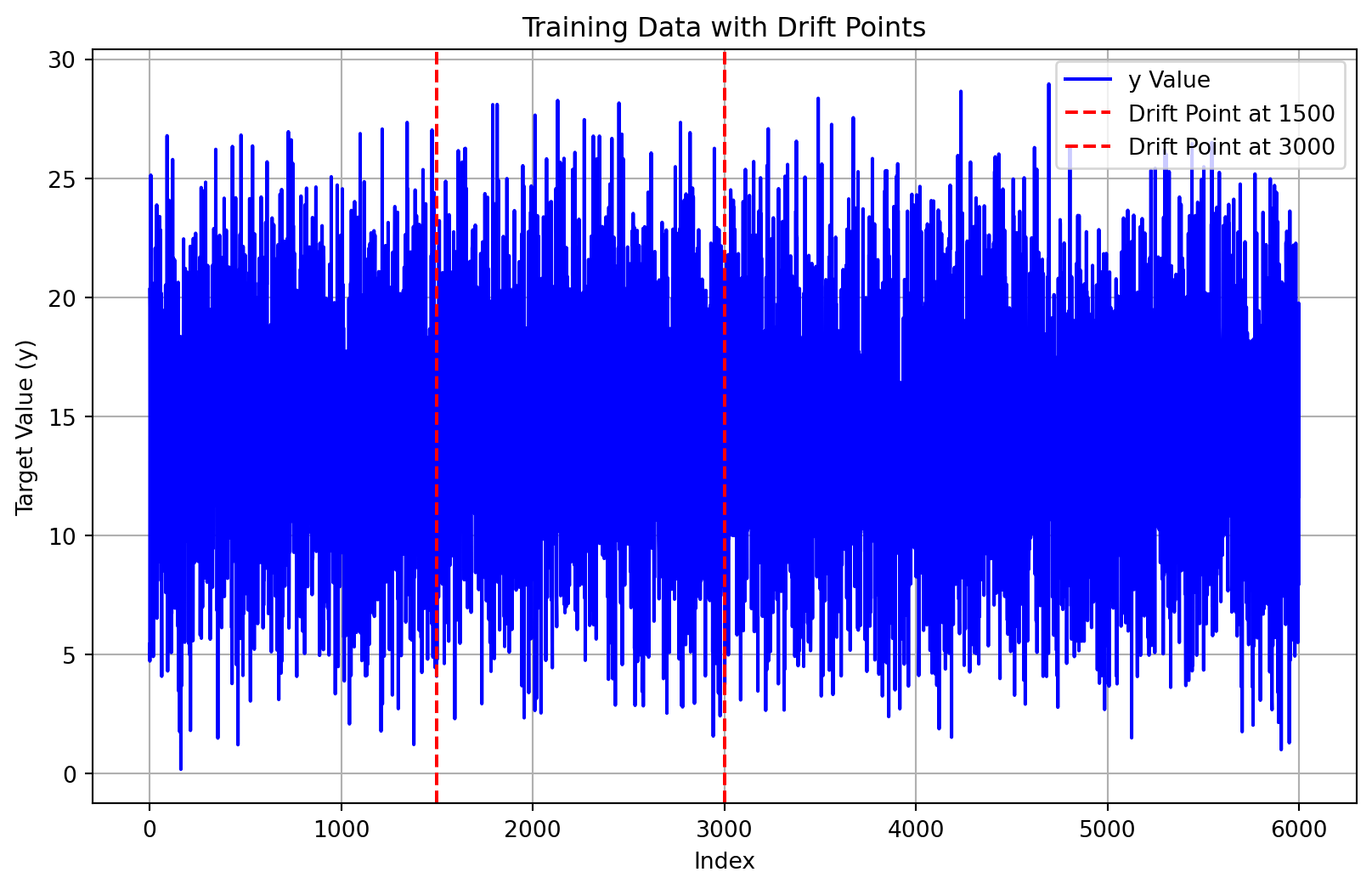

plot_data_with_drift_points(test, target_column, n_train, title="Testing Data with Drift Points")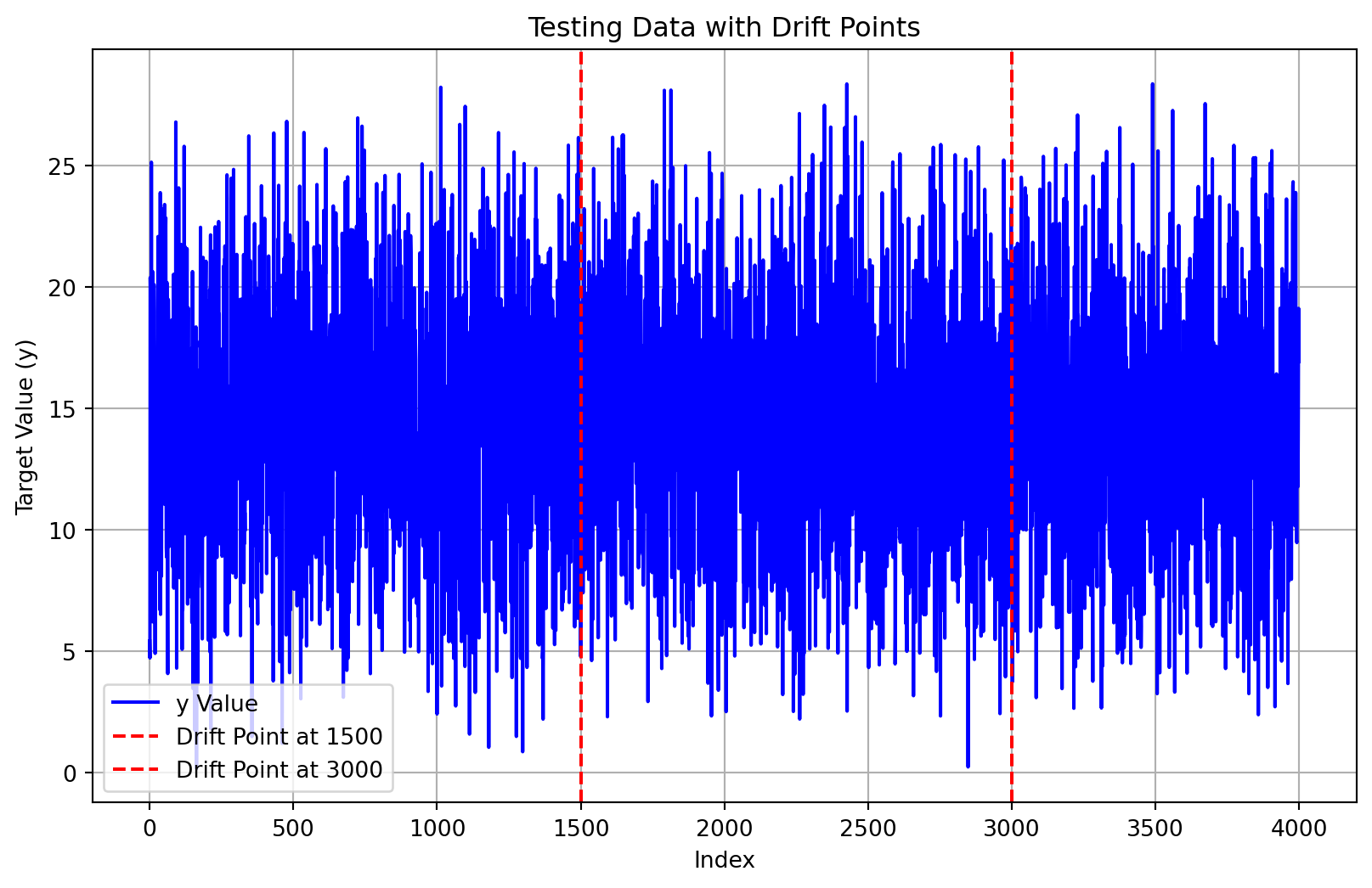

E.2.2 The Friedman Drift Data Set from spotpython

A data generator for the Friedman Drift dataset is implemented in the spotpython package, see friedman.py. The spotpython version is a simplified version of the river implementation. The spotPyton version allows the generation of constant input values for the features. This is useful for visualizing the concept drifts. For the productive use the river version should be used.

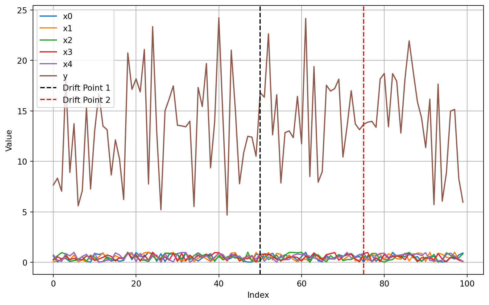
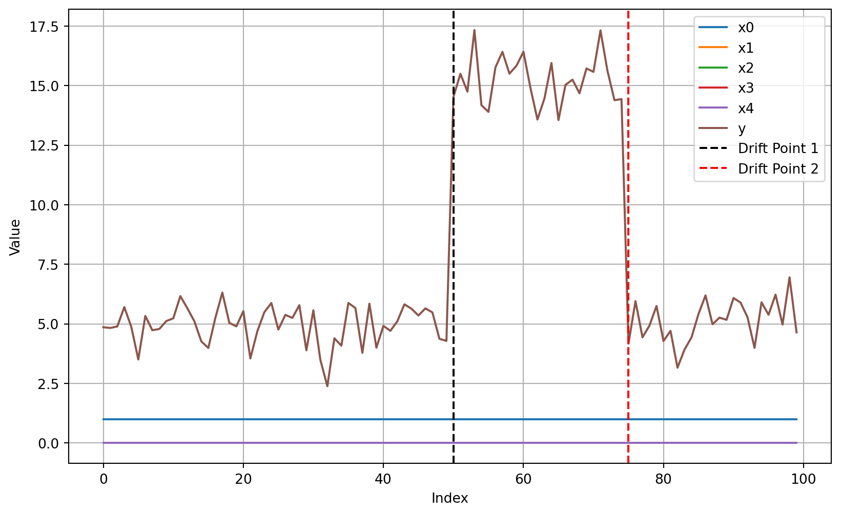
Plotting the first 100 samples of the Friedman Drift dataset, we can not see the concept drifts at \(p_1\) and \(p_2\). Drift can be visualized by plotting the target values over time for constant features, e,g, if \(x_0\) is set to \(1\) and all other features are set to \(0\). This is illustrated in the following plot.

from spotpython.data.friedman import FriedmanDriftDataset

def plot_friedman_drift_data(n_samples, seed, change_point1, change_point2, constant=True):
    data_generator = FriedmanDriftDataset(n_samples=n_samples, seed=seed, change_point1=change_point1, change_point2=change_point2, constant=constant)
    data = [data for data in data_generator]
    indices = [i for _, _, i in data]
    values = {f"x{i}": [] for i in range(5)}
    values["y"] = []
    for x, y, _ in data:
        for i in range(5):
            values[f"x{i}"].append(x[i])
        values["y"].append(y)

    plt.figure(figsize=(10, 6))
    for label, series in values.items():
        plt.plot(indices, series, label=label)
    plt.xlabel('Index')
    plt.ylabel('Value')
    plt.axvline(x=change_point1, color='k', linestyle='--', label='Drift Point 1')
    plt.axvline(x=change_point2, color='r', linestyle='--', label='Drift Point 2')
    plt.legend()
    plt.grid(True)
    plt.show()

plot_friedman_drift_data(n_samples=100, seed=42, change_point1=50, change_point2=75, constant=False)
plot_friedman_drift_data(n_samples=100, seed=42, change_point1=50, change_point2=75, constant=True)

Friedman, Jerome H. 1991. “Multivariate Adaptive Regression Splines.” The Annals of Statistics 19 (1): 1–67.

Ikonomovska, Elena, João Gama, and Sašo Džeroski. 2011. “Learning Model Trees from Evolving Data Streams.” Data Mining and Knowledge Discovery 23 (1): 128–68.