import torch
import torch.nn as nn
import torch.optim as optim
import numpy as np
import matplotlib.pyplot as plt
import torchdiffeq50 Neural ODEs
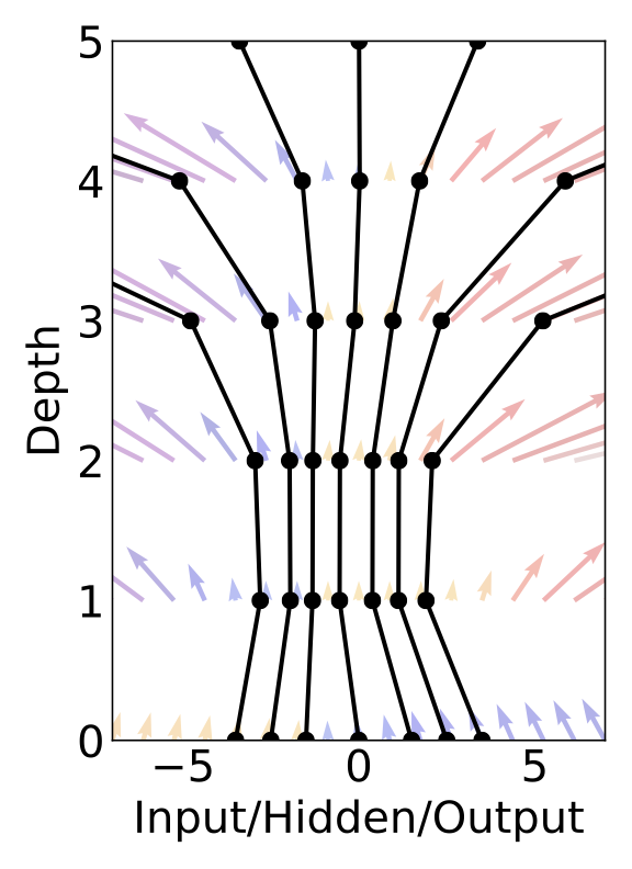
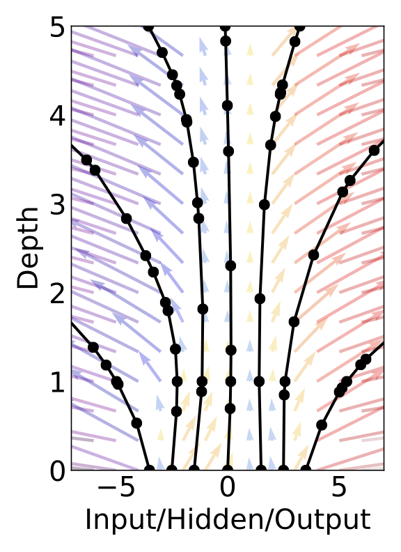
Neural ODEs are related to Residual Neural Networks (ResNets). We consider ResNets in Section 49.1.
50.1 Neural Ordinary Differential Equations
Neural Ordinary Differential Equations (Neural ODEs) are a class of models that are based on ordinary differential equations (ODEs). They are a generalization of ResNets, where the depth of the network is treated as a continuous parameter. Neural ODEs have been introduced by Chen et al. (2018). We will consider dynamical systems first.
Definition 50.1 A dynamical system is a triple \[ (\mathcal{S}, \mathcal{T}, \Phi) \] where
- \(\mathcal{S}\) is the state space
- \(\mathcal{T}\) is the parameter space, and
- \(\Phi: (\mathcal{T} \times \mathcal{S}) \longrightarrow \mathcal{S}\) is the evolution.
Definition 50.1 is a very general definition that includes all sort of dynamical systems. We deal with ODEs where \(\Phi\) plays the role of the general solution: indeed a 1-parameter family of transformations of the state space. \(\mathcal{T}=\mathbb{R}_{+}\) is the time, and usually, \(\mathcal{S}=\mathbb{R}^{n}\) is the state space. The evolution takes a point in space (initial value), a point in time, and returns the a point in space. A general solution to an ODE is a function \(y: I \times \mathbb{R}^{n} ⟶ \mathbb{R}^{n}\): a 1-parameter (usually time is the parameter) family of transformations of the state space. A 1-parameter family of transformations is often called a flow.
First-order Ordinary Differential Equations (ODEs) can be defined as follows:
Definition 50.2 (First-Order Ordinary Differential Equation (ODE)) \[ \mathbf{\dot{y}}(t) = f(t, \mathbf{y}(t)),\quad \mathbf{y}(t_0) = y_0,\quad f: \mathbb{R} \times \mathbb{R}^n \to \mathbb{R}^n \]
The solution of the ODE is the function \(\mathbf{y}(t)\) that satisfies the ODE and the initial condition, which can be stated as an initial value problems (IVP), i.e. predict \(\mathbf{y}(t_1)\) given \(\mathbf{y}(t_0)\).
Definition 50.3 (Initial Value Problem (IVP)) \[ \mathbf{y}(t_1) = \mathbf{y}(t_0) + \int_{t_0}^{t_1} f(\mathbf{y}(t), t) \mathrm{d}t = \textrm{ODESolve}(\mathbf{y}(t_0), f, t_0, t_1) \tag{50.1}\]
The existence and uniqueness of solutions to an IVP is ensured by the Picard-Lindelöf theorem, provided the RHS of the ODE is Lipschitz continuous. Lipschitz continuity is a property that pops up quite often in ODE-related results in ML.
Definition 50.4 (Lipschitz Continuity) A function \(f: X \subset \mathbb{R}^{n} ⟶ \mathbb{R}^{n}\) is called Lipschitz continuous (with constant \(\lambda\)) if
\[ || f(x_{1}) - f(x_{2}) || \leq \lambda ||x_{1} - x_{2}|| \quad \forall x_{1},x_{2} \in X. \]
Note that Lipschitz continuity is a stronger condition than just continuity.
Numerical solvers can be used to perform the forward pass and solve the IVP. If we use, for example, Euler’s method, we have the following update rule:
\[ \mathbf{y}(t+h) = \mathbf{y}(t) + hf(\mathbf{y}(t), t) \tag{50.2}\]
where \(h\) is the step size. The update rule is applied iteratively to solve the IVP. The solution is a discrete approximation of the continuous function \(\mathbf{y}(t)\).
Equation 50.2 looks almost identical to a ResNet block (see Equation 49.1). This was one of the main motivations for Neural ODEs (Chen et al. 2018).
ResNets update hidden states by employing residual connections:
\[ \mathbf{y}_{l+1} = \mathbf{y}_l + f(\mathbf{y}_l, \theta_l) \]
where \(f\) is a neural network with parameters \(\theta_l\), and \(\mathbf{y}_l\) and \(\mathbf{y}_{l+1}\) are the hidden states at subsequent layers, \(l \in \{0, \ldots, L\}\).
These updates can be seen as Euler discretizations of continuous transformations.
\[\begin{align} \mathbf{\dot{y}} &= f(\mathbf{y}, t, \theta) \\ &\Bigg\downarrow \ \textrm{Euler Discretization} \\ \mathbf{y}_{n+1} &= \mathbf{y}_n + h f(\mathbf{y}_n, t_n, \theta) \end{align}\]
What happens in a residual network (with step sizes \(h\)) if we consider the continuous limit of each discrete layer in the network? What happens as we add more layers and take smaller steps? The answer seems rather astounding: instead of having a discrete number of layers between the input and output domains, we allow the evolution of the hidden states to become continuous.


The main technical difficulty in training continuous-depth networks is performing backpropagation through the ODE solver. Differentiating through the operations of the forward pass is straightforward, but incurs a high memory cost and introduces additional numerical error.
Pontryagin (1987) treated the ODE solver as a black box, and computed gradients using the adjoint sensitivity method. This approach computes gradients by solving a second, augmented ODE backwards in time, and is applicable to all ODE solvers. It scales linearly with problem size, has low memory cost, and explicitly controls numerical error.
Consider optimizing a scalar-valued loss function \(L()\), whose input is the result of an ODE solver: \[ L(y(t_1) = L \left(y(t_0) + \int_{t_0}^{t_1} f(y(t), t, \theta) dt \right) = L \left( \textrm{ODESolve}( y(t_0), f, t_0, t_1, \theta) \right) \tag{50.3}\]
Equation 50.3 is related to {Equation 50.1}. To optimize \(L\), we require gradients with respect to \(\theta\).
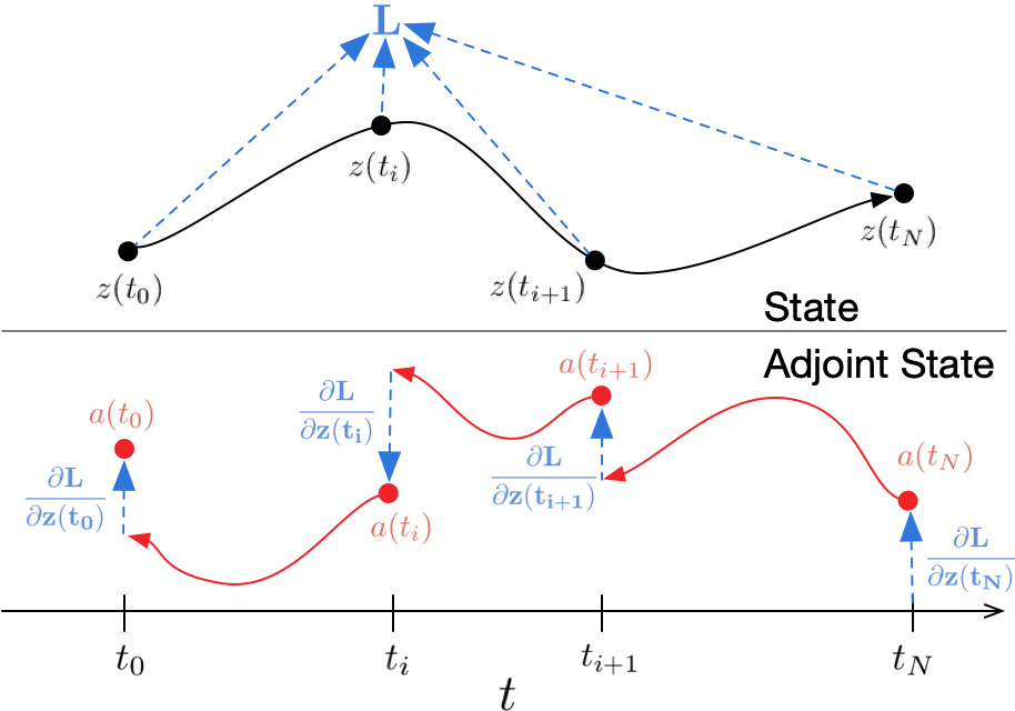
Similar to standard neural networks, we start with determining how the gradient of the loss depends on the hidden state \(y(t)\) at each instant. This quantity is called the adjoint \(a(t) = \frac{\partial{L}}{\partial y(t)}\). It satisfies the following IVP:
\[ \dot{\mathbf{a}}(t) = -\mathbf{a}(t)^{\top} \frac{\partial f(\mathbf{x}(t), t, \theta)}{\partial \mathbf{x}}, \quad \mathbf{a}(t_1) = \frac{\partial L}{\partial \mathbf{x}(t_1)}. \]
Its dynamics are given by another ODE, which can be thought of as the instantaneous analog of the chain rule: \[ \frac{d a(t)}{d t} = - a(t)^{T} \frac{\partial f(y(t), t, \theta)}{\partial y}. \]
Thus, starting from the initial (remember we are running backwards) value \(\mathbf{a}(t_1) = \frac{\partial L}{\partial \mathbf{x}(t_1)}\), we can compute \(\mathbf{a}(t_0) = \frac{\partial L}{\partial \mathbf{x}(t_0)}\) by another call to an ODE solver.
Finally, computing the gradients with respect to the parameters \(\theta\) requires evaluating a third integral, which depends on both \(\mathbf{x}(t)\) and \(\mathbf{a}(t)\):
\[ \frac{\mathrm{d}L}{\mathrm{d}\theta} = -\int_{t_1}^{t_0} \mathbf{a}(t)^{\top}\frac{\partial f}{\partial \theta} \mathrm{d}t, \]
So this method trades off computation for memory—in fact the memory requirement for this gradient calculation is only \(\mathcal{O}(1)\) with respect to the number of layers. The corresponding algorithm is described in Chen et al. (2018), see also Figure 50.3.

Here you can find a very good explanation of the following result based on Lagrange multipliers.
50.2 Regression Example
To illustrate this concept, we will consider a simple regression example. This example is based on the Neural-ODEs tutorial from Neural Ordinary Differential Equations, which is provided by Chen et al. (2018). We will use the ODE solvers from Torchdiffeq.
Neural ODEs, or ODE-Nets, build complex models by chaining together simple building blocks, similar to residual networks. Here, our base layer will define the dynamics of an ODE, which will be interconnected using an ODE solver to form the complete neural network model.
50.2.1 Specifying the Dynamics Layer
The dynamics of an ODE can be captured by the equation:
\[ \dot y(t) = f(y(t), t, \theta), \qquad y(0) = y_0, \] where the initial value \(y_0 \in \mathbb{R}^n\). The \(\theta\) parameters were added to the dynamics, so the dynamics function has the dimensions \(f : \mathbb{R}^{n} \times \mathbb{R} \times \mathbb{R}^{|\theta|} \to \mathbb{R}^n\), where \(|\theta|\) is the number of parameters we’ve added to \(f\).
We need the dynamics function to take in the current state \(y(t)\) of the ODE, the current time \(t\), and some parameters \(\theta\), and output \(\frac{\partial y(t)}{\partial t}\), which has the same shape as \(y(t)\). They are passed as input to a multi-layer perceptron (MLP). Multiple evaluations of this dynamics layer can be combined using any suitable ODE solver, such as the adaptive-step Dormand-Price solver implemented in the torchdiffeq library’s odeint function.
Let’s start by defining an MLP class to serve as the building block of our models.
class MLP(nn.Module):
    def __init__(self, layer_sizes):
        super(MLP, self).__init__()
        layers = []
        for i in range(len(layer_sizes) - 1):
            layers.append(nn.Linear(layer_sizes[i], layer_sizes[i+1]))
            if i < len(layer_sizes) - 2:
                layers.append(nn.Tanh())
        self.network = nn.Sequential(*layers)

    def forward(self, x):
        return self.network(x)
Next, we’ll define a ResNet class that uses the MLP as its inner component.
class ResNet(nn.Module):
    def __init__(self, layer_sizes, depth):
        super(ResNet, self).__init__()
        self.mlp = MLP(layer_sizes)
        self.depth = depth

    def forward(self, x):
        for _ in range(self.depth):
            x = self.mlp(x) + x
return xODEFuncdefines how the system evolves over time using the MLP to approximate derivatives \(\dot{y}(t)\).ODEBlockspecifies the network structure. It usestorchdiffeq.odeintto integrate these dynamics over time.
class ODEFunc(nn.Module):
    def __init__(self, layer_sizes):
        super(ODEFunc, self).__init__()
        self.mlp = MLP(layer_sizes)

    def forward(self, t, y):
        t_expanded = t.expand_as(y)
        state_and_time = torch.cat([y, t_expanded], dim=1)
        return self.mlp(state_and_time)

class ODEBlock(nn.Module):
    def __init__(self, odefunc):
        super(ODEBlock, self).__init__()
        self.odefunc = odefunc

    def forward(self, x):
        t = torch.tensor([0.0, 1.0])
        out = torchdiffeq.odeint(self.odefunc, x, t, atol=1e-3, rtol=1e-3)
        return out[1]
Generate a toy 1D dataset.
inputs = torch.linspace(-2.0, 2.0, 10).reshape(10, 1)
targets = inputs**3 +  0.1 * inputs
We specify the hyperparameters for the ResNet and ODE-Net.
layer_sizes = [1, 25, 1]
param_scale = 1.0
step_size = 0.01
train_iters = 1000
resnet_depth = 3
Initialize and train the ResNet.
resnet = ResNet(layer_sizes, resnet_depth)
criterion = nn.MSELoss()
optimizer = optim.SGD(resnet.parameters(), lr=step_size)

for _ in range(train_iters):
    optimizer.zero_grad()
    outputs = resnet(inputs)
    loss = criterion(outputs, targets)
    loss.backward()
    optimizer.step()
# We need to change the input dimension to 2, to allow time-dependent dynamics.
odenet_layer_sizes = [2, 25, 1]
# Initialize and train ODE-Net.
odefunc = ODEFunc(odenet_layer_sizes)
odenet = ODEBlock(odefunc)
optimizer = optim.SGD(odenet.parameters(), lr=step_size)
for _ in range(train_iters):
optimizer.zero_grad()
outputs = odenet(inputs)
loss = criterion(outputs, targets)
loss.backward()
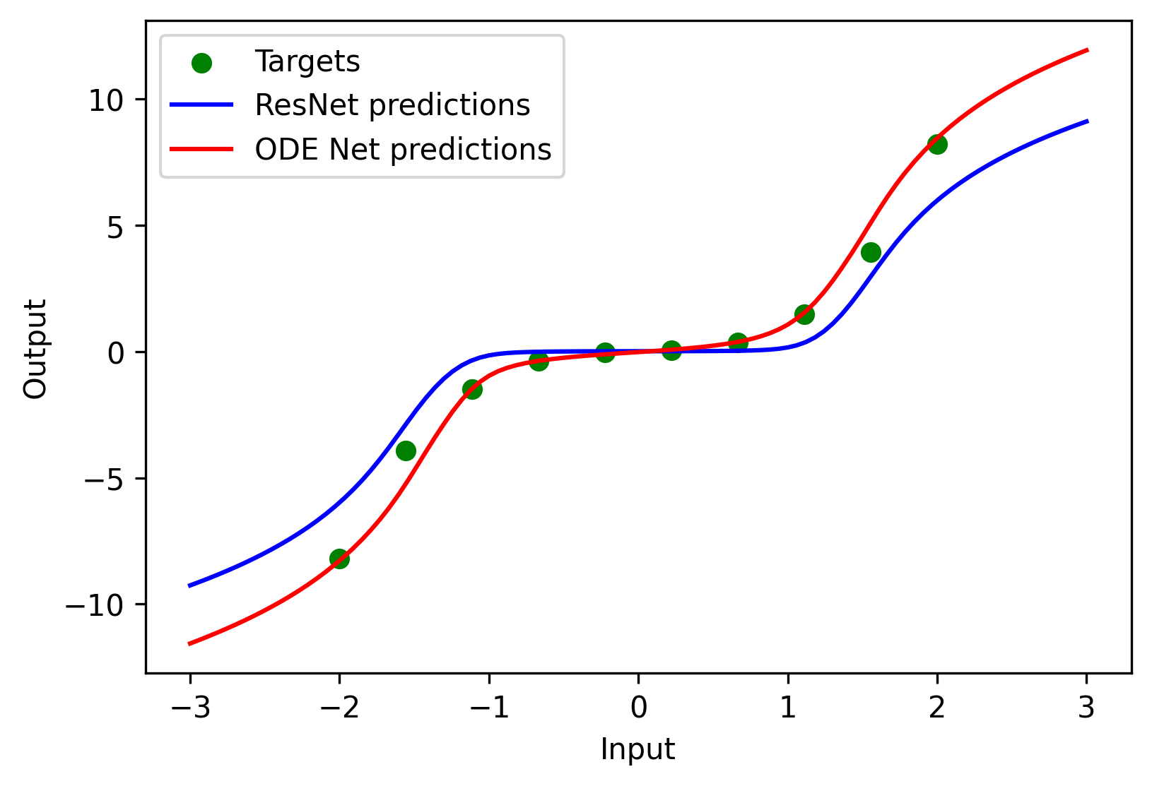
optimizer.step()Finally, plot the predictions of both models.
fine_inputs = np.linspace(-3.0, 3.0, 100).reshape(-1, 1)
fine_inputs_tensor = torch.from_numpy(fine_inputs).float()
plt.figure(figsize=(6, 4), dpi=150)
plt.scatter(inputs, targets, color='green', label='Targets')
plt.plot(fine_inputs, resnet(fine_inputs_tensor).detach().numpy(), color='blue', label='ResNet predictions')

plt.plot(fine_inputs, odenet(fine_inputs_tensor).detach().numpy(), color='red', label='ODE Net predictions')
plt.xlabel('Input')
plt.ylabel('Output')
plt.legend()
plt.show()
50.3 Further Reading
Neural ODEs have received a lot of attention in the past few years, ever since their introduction in Neurips 2018. Some of many many work in this field include:
- Neural Stochastic Differential Equations (Neural SDEs),
- Neural Controlled Differential Equations (Neural CDEs),
- Graph ODEs,
- Hamiltonial Neural Networks, and
- Lagrangian Neural Networks.
Michael Poli maintains the excellent Awesome Neural ODE, a collection of resources regarding the interplay between neural differential equations, dynamical systems, deep learning, control, numerical methods and scientific machine learning.
Torchdyn is an excellent library for Neural Differential Equations.
Implicit Layers is a list of tutorials on implicit functions and automatic differentiation, Neural ODEs, and Deep Equilibrium Models.
Understanding Neural ODE’s is an excellent blogpost on ODEs and Neural ODEs.
Patrick Kidger’s doctoral dissertation is an excellent textbook on Neural Differential Equations, see Kidger (2022).