[20]{.chapter-number}  [Classification]{.chapter-title}

doi:10.48550/arXiv.2307.10262

20 Classification

In classification we have a qualitative response variable.

Figure 20.1: Classification. Taken from James et al. (2014)

Here the response variable \(Y\) is qualitative, e.g., email is one of \(\cal{C} = (spam, ham)\), where ham is good email, digit class is one of \(\cal{C} = \{ 0, 1, \ldots, 9 \}\). Our goals are to:

Build a classifier \(C(X)\) that assigns a class label from \(\cal{C}\) to a future unlabeled observation \(X\).
Assess the uncertainty in each classification
Understand the roles of the different predictors among \(X = (X_1,X_2, \ldots, X_p)\).

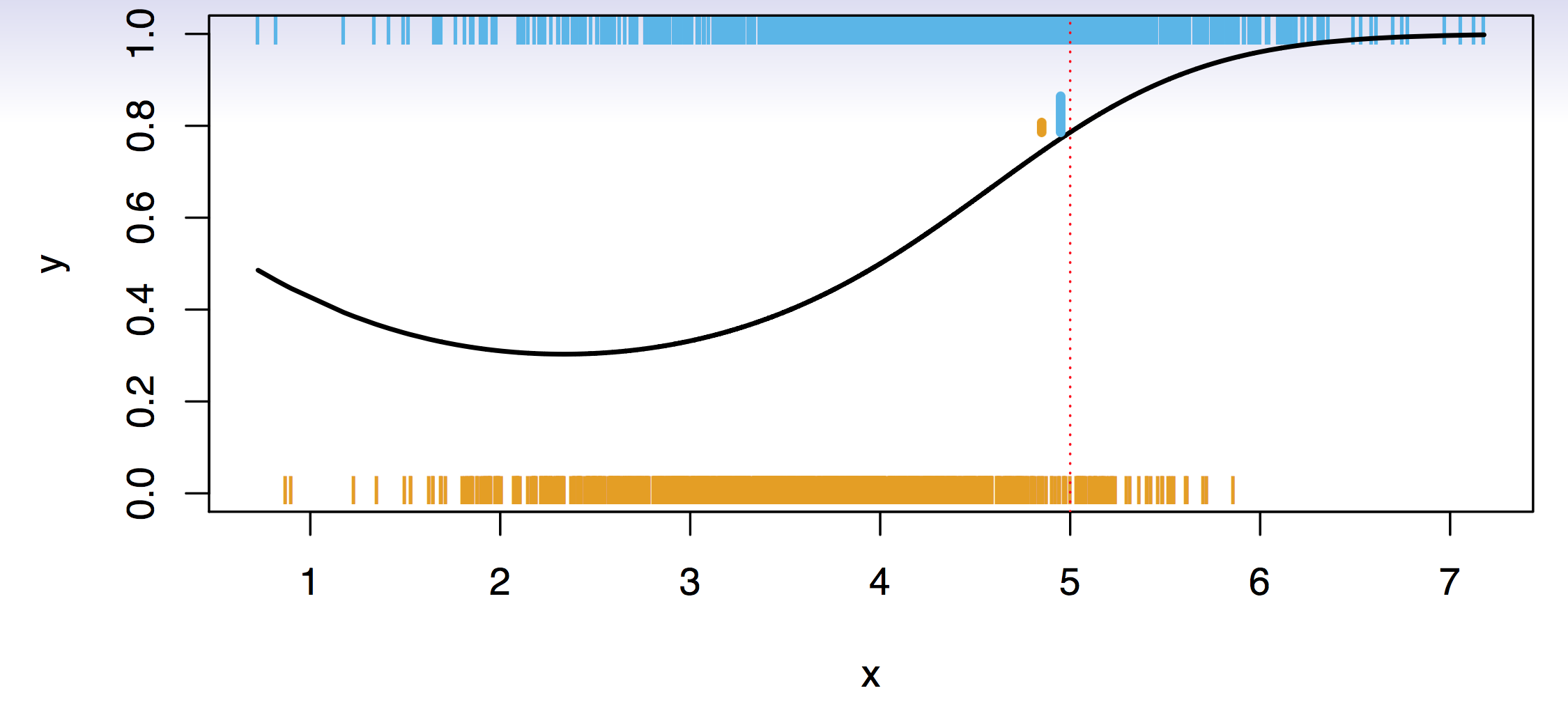
Simulation example depicted in@fig-0218a. \(Y\) takes two values, zero and one, and \(X\) has only one value. Big sample: each single vertical bar indicates an occurrance of a zero (orange) or one (blue) as a function of the \(X\)s. Black curve generated the data: it is the probability of generating a one. For high values of \(X\), the probability of ones is increasing. What is an ideal classifier \(C(X)\)?

Suppose the \(K\) elements in \(\cal{C}\) are numbered \(1,2,\ldots, K\). Let \[ p_k(x) = Pr(Y = k|X = x), k = 1,2,\ldots,K. \]

These are the conditional class probabilities at \(x\); e.g. see little barplot at \(x = 5\). Then the Bayes optimal classifier at \(x\) is \[ C(x) = j \qquad \text{ if } p_j(x) = \max \{p_1(x),p_2(x),\ldots, p_K(x)\}. \] At \(x=5\) there is an 80% probability of one, and an 20% probability of a zero. So, we classify this point to the class with the highest probability, the majority class.

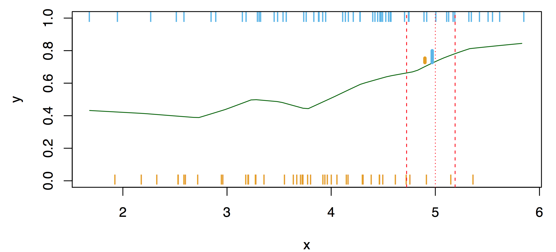
Nearest-neighbor averaging can be used as before. This is illustrated in Fig.~\(\ref{fig:0219a}\). Here, we consider 100 points only. Nearest-neighbor averaging also breaks down as dimension grows. However, the impact on \(\hat{C}(x)\) is less than on \(\hat{p}_k (x)\), \(k = 1, \ldots, K\).

Figure 20.2: Classification. Taken from James et al. (2014)

20.1 Classification: Some Details

Average number of errors made to measure the performance. Typically we measure the performance of \(\hat{C}(x)\) using the misclassification error rate: \[ Err_{Te} = Ave_{i\in Te} I[y_i \neq \hat{C} (x_i) ]. \] The Bayes classifier (using the true \(p_k(x)\)) has smallest error (in the population).

20.2 k-Nearest Neighbor Classification

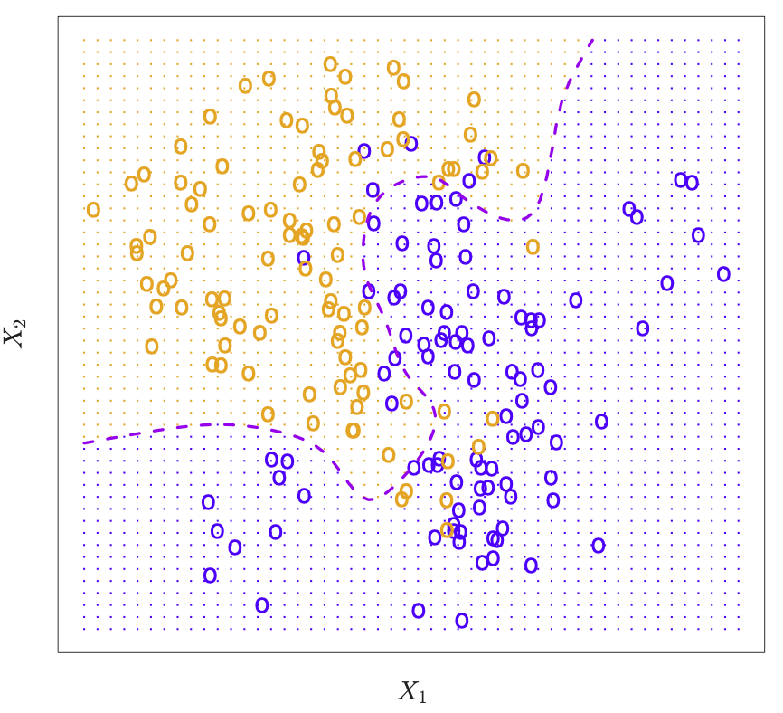
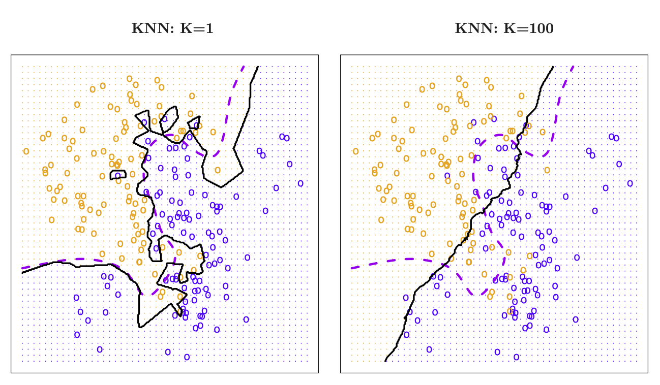
Consider k-nearest neighbors in two dimensions. Orange and blue dots label the true class memberships of the underlying points in the 2-dim plane. Dotted line is the decision boundary, that is the contour with equal probability for both classes.

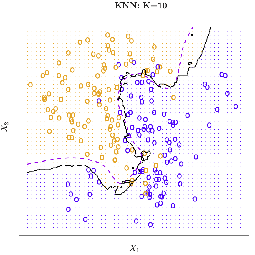
Nearest-neighbor averaging in 2-dim. At any given point we want to classify, we spread out a little neighborhood, say \(K=10\) points from the neighborhood and calulated the percentage of blue and orange. We assign the color with the highest probability to this point. If this is done for every point in the plane, we obtain the solid black curve as the esitmated decsion boundary.

We can use \(K=1\). This is the nearest-neighbor classifier. The decision boundary is piecewise linear. Islands occur. Approximation is rather noisy.

\(K=100\) leads to a smooth decision boundary. But gets uninteresting.

Figure 20.3: K-nearest neighbors in two dimensions. Taken from James et al. (2014)

Figure 20.4: K-nearest neighbors in two dimensions. Taken from James et al. (2014)

Figure 20.5: K-nearest neighbors in two dimensions. Taken from James et al. (2014)

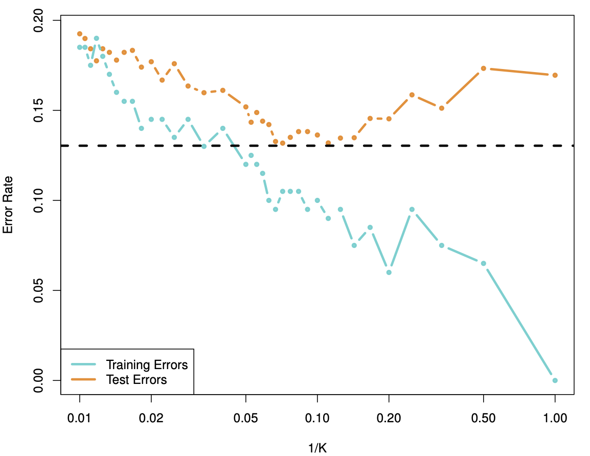
\(K\) large means higher bias, so \(1/K\) is chosen, because we go from low to high complexity on the \(x\)-error, see Figure 20.6. Horizontal dotted line is the base error.

Figure 20.6: K-nearest neighbors classification error. Taken from James et al. (2014)

20.2.1 Minkowski Distance

The Minkowski distance of order \(p\) (where \(p\) is an integer) between two points \(X=(x_1,x_2,\ldots,x_n)\text{ and }Y=(y_1,y_2,\ldots,y_n) \in \mathbb{R}^n\) is defined as: \[ D \left( X,Y \right) = \left( \sum_{i=1}^n |x_i-y_i|^p \right)^\frac{1}{p}. \]