24  Kriging with spotPython based on the Forrester et al. textbook

This chapter xplains how the spotpython Kriging class implements standard formulas from Forrester et al. (Engineering Design via Surrogate Modelling), focusing on Chapters 2, 3, and 6 (Gaussian process/Kriging modelling, likelihood-based hyperparameter estimation, prediction, and expected improvement).

24.1 High-level model and notation

• Training data: X ∈ R^{n×k}, y ∈ R^n.
• Correlation model: R(i,j) = exp(-∑_d θ_d · (x_i,d − x_j,d)^2) for ordered/numeric variables; factor variables use a categorical distance with the same exp(-D) envelope. θ are in log10 in this code, internally exponentiated as 10^θ.
• Nugget: λ ≥ 0 (also in log10 here, exponentiated as 10^λ). Interpolation uses eps (tiny) instead of λ; regression uses λ; reinterpolation uses a λ→ε adjustment during prediction variance.
• Mean function: constant mean μ (ordinary Kriging).
• Concentrated likelihood (Forrester): given R (n×n) and residual variance σ^2 = (r^T R^{-1} r)/n with r = y − 1·μ and μ = (1^T R^{-1} y)/(1^T R^{-1} 1), the concentrated negative log-likelihood is n/2·log(σ^2) + 1/2·log|R| (constants dropped).

24.2 Correlation matrix build: build_Psi()

• Psi is the correlation matrix R (without the nugget) from pairwise distances:
  • Ordered/numeric variables use squared Euclidean dist weighted by 10^θ.
  • Factor variables use a categorical metric (metric_factorial).
  • Final Psi = exp(−D).
• The method returns the upper triangle; the full R is formed later as R = Psi + Psi^T + I (and + λI if applicable).

Code mapping:

def build_Psi(self) -> None:
    n, k = self.X_.shape
    theta10 = self._get_theta10_from_logtheta()  # 10**theta, isotropic expands to k
    Psi = np.zeros((n, n), dtype=np.float64)

    if self.ordered_mask.any():
        X_ordered = self.X_[:, self.ordered_mask]
        D_ordered = squareform(
            pdist(X_ordered,
            metric="sqeuclidean",
            w=theta10[self.ordered_mask]))
        Psi += D_ordered

    if self.factor_mask.any():
        X_factor = self.X_[:, self.factor_mask]
        D_factor = squareform(
            pdist(X_factor, metric=self.metric_factorial,
            w=theta10[self.factor_mask]))
        Psi += D_factor

    Psi = np.exp(-Psi)                 # R = exp(-D)
    return np.triu(Psi, k=1)           # upper triangle only

24.3 Likelihood and hyperparameters: likelihood()

• Input x packs [log10 θ] plus, for regression/reinterpolation, log10 λ, and optionally p exponents (if enabled).
• The method:
  1. Forms R = (upper + transpose) + I + λI (with λ = 10^logλ; for interpolation λ := eps).
  2. Cholesky factorization R = U U^T.
  3. μ = (1^T R^{-1} y)/(1^T R^{-1} 1) via triangular solves with U.
  4. σ^2 = (r^T R^{-1} r)/n with r = y − 1·μ.
  5. −log L = n/2·log(σ^2) + 1/2·log|R|, with log|R| = 2·∑ log diag(U).

Code mapping (directly implements the standard concentrated likelihood):

def likelihood(self, x: np.ndarray) -> Tuple[float, np.ndarray, np.ndarray]:
    X = self.X_; y = self.y_.flatten()
    self.theta = x[: self.n_theta]

    if (self.method == "regression") or (self.method == "reinterpolation"):
        lambda_ = 10.0**x[self.n_theta : self.n_theta + 1]   # nugget on linear scale
        if self.optim_p:
            self.p_val = x[self.n_theta + 1 : self.n_theta + 1 + self.n_p]
    elif self.method == "interpolation":
        lambda_ = self.eps
        if self.optim_p:
            self.p_val = x[self.n_theta : self.n_theta + self.n_p]

    n = X.shape[0]; one = np.ones(n)
    Psi_up = self.build_Psi()
    Psi = Psi_up + Psi_up.T + np.eye(n) + np.eye(n) * lambda_  # R = corr + I + λI

    U = np.linalg.cholesky(Psi)
    LnDetPsi = 2.0 * np.sum(np.log(np.abs(np.diag(U))))        # log|R|

    # R^{-1}y and R^{-1}1 via triangular solves
    temp_y  = np.linalg.solve(U, y);   vy   = np.linalg.solve(U.T, temp_y)
    temp_1  = np.linalg.solve(U, one); vone = np.linalg.solve(U.T, temp_1)

    mu = (one @ vy) / (one @ vone)
    resid = y - one * mu
    tresid = np.linalg.solve(U, resid); tresid = np.linalg.solve(U.T, tresid)
    SigmaSqr = (resid @ tresid) / n

    negLnLike = (n / 2.0) * np.log(SigmaSqr) + 0.5 * LnDetPsi
    return negLnLike, Psi, U

24.4 Hyperparameter optimization: max_likelihood()

• Minimizes the concentrated negative log-likelihood over [log10 θ, log10 λ, p] using differential evolution.
• Objective = likelihood(x)[0].
• Bounds are assembled in fit() depending on method and options.

Code mapping:

def max_likelihood(self, bounds: List[Tuple[float, float]]) -> Tuple[np.ndarray, float]:
    def objective(logtheta_loglambda_p_: np.ndarray) -> float:
        neg_ln_like, _, _ = self.likelihood(logtheta_loglambda_p_)
        return neg_ln_like

    result = differential_evolution(func=objective, bounds=bounds, seed=self.seed)
    return result.x, result.fun

24.5 Model fitting workflow: fit()

• Sets k, n, variable type masks; selects n_theta (1 if isotropic else k).
• Builds bounds:
  • interpolation: k θ-bounds only.
  • regression/reinterpolation: k θ-bounds + 1 λ-bound.
  • If optim_p: adds p-bounds (n_p entries).
• Calls max_likelihood to obtain best x = [log10 θ, log10 λ, p].
• Stores:
  • theta = first n_theta entries of x.
  • Lambda = next 1 entry (for regression/reinterpolation) — kept on log10 scale in the model’s state; transformed to linear only inside likelihood/_pred.
  • p_val if enabled.
• Computes final Psi, U and negLnLike at the found hyperparameters.

Code mapping:

def fit(self,
        X: np.ndarray,
        y: np.ndarray,
        bounds: Optional[List[Tuple[float, float]]] = None) -> "Kriging":
    X = np.asarray(X); y = np.asarray(y).flatten()
    self.X_, self.y_ = X, y
    self.n, self.k = self.X_.shape
    self._set_variable_types()
    if self.n_theta is None: self._set_theta()
    self.min_X = np.min(self.X_, axis=0); self.max_X = np.max(self.X_, axis=0)

    if bounds is None:
        if self.method == "interpolation":
            bounds = [(self.min_theta, self.max_theta)] * self.k
        else:
            bounds = [(self.min_theta, self.max_theta)] * self.k + 
                      (self.min_Lambda, self.max_Lambda)]
    if self.optim_p:
        bounds += [(self.min_p, self.max_p)] * self.n_p

    self.logtheta_loglambda_p_, _ = self.max_likelihood(bounds)

    self.theta = self.logtheta_loglambda_p_[: self.n_theta]
    if (self.method == "regression") or (self.method == "reinterpolation"):
        self.Lambda = self.logtheta_loglambda_p_[self.n_theta : self.n_theta + 1]
        if self.optim_p:
            self.p_val = self.logtheta_loglambda_p_[self.n_theta + 1 : self.n_theta + 1 + self.n_p]
    elif self.method == "interpolation":
        self.Lambda = None
        if self.optim_p:
            self.p_val = self.logtheta_loglambda_p_[self.n_theta : self.n_theta + self.n_p]

    self.negLnLike, self.Psi_, self.U_ = self.likelihood(self.logtheta_loglambda_p_)
    self._update_log()
    return self

24.6 Correlation vector for a new point: build_psi_vec()

• For a new x ∈ R^k, compute ψ(x) ∈ R^n with ψ_i = exp(−D(x, x_i)), using same distance construction and weights 10^θ as for R.

Code mapping:

def build_psi_vec(self, x: np.ndarray) -> None:
    n = self.X_.shape[0]
    theta10 = self._get_theta10_from_logtheta()
    D = np.zeros(n)

    if self.ordered_mask.any():
        X_ordered = self.X_[:, self.ordered_mask]
        x_ordered = x[self.ordered_mask]
        D += cdist(x_ordered.reshape(1, -1), X_ordered, metric="sqeuclidean", w=theta10[self.ordered_mask]).ravel()

    if self.factor_mask.any():
        X_factor = self.X_[:, self.factor_mask]
        x_factor = x[self.factor_mask]
        D += cdist(x_factor.reshape(1, -1), X_factor, metric=self.metric_factorial, w=theta10[self.factor_mask]).ravel()

    psi = np.exp(-D)                  # ψ(x)
    return psi

24.7 Prediction at a new x: _pred() and predict()

• Ordinary Kriging predictor (Forrester):
  • Mean μ and R^{-1} reused (via stored U).
  • Predictor: f(x) = μ + ψ(x)^T R^{-1} (y − 1·μ).
  • Predictive variance s^2(x) depends on method:
    • interpolation/regression: s^2(x) = σ^2 [1 + λ − ψ(x)^T R^{-1} ψ(x)].
    • reinterpolation: uses R_adj = R − λI + εI for the variance term, consistent with a reinterpolation/nugget-adjusted scheme.
• Expected improvement (EI): computed when requested using standard normal CDF/PDF via erf; the code returns negative EI for minimization.

Code mapping:

def _pred(self, x: np.ndarray) -> float:
    y = self.y_.flatten()
    # load θ, λ (λ transformed to linear scale), p
    if (self.method == "regression") or (self.method == "reinterpolation"):
        self.theta = self.logtheta_loglambda_p_[: self.n_theta]
        lambda_ = 10.0**self.logtheta_loglambda_p_[self.n_theta : self.n_theta + 1]
        if self.optim_p:
            self.p_val = self.logtheta_loglambda_p_[self.n_theta + 1 : self.n_theta + 1 + self.n_p]
    elif self.method == "interpolation":
        self.theta = self.logtheta_loglambda_p_[: self.n_theta]
        lambda_ = self.eps

    U = self.U_; n = self.X_.shape[0]; one = np.ones(n)

    # μ and R^{-1}r
    y_tilde = np.linalg.solve(U, y); y_tilde = np.linalg.solve(U.T, y_tilde)
    one_tilde = np.linalg.solve(U, one); one_tilde = np.linalg.solve(U.T, one_tilde)
    mu = (one @ y_tilde) / (one @ one_tilde)

    resid = y - one * mu
    resid_tilde = np.linalg.solve(U, resid); resid_tilde = np.linalg.solve(U.T, resid_tilde)

    psi = self.build_psi_vec(x)

    # σ^2 and s^2(x)
    SigmaSqr = (resid @ resid_tilde) / n
    psi_tilde = np.linalg.solve(U, psi); psi_tilde = np.linalg.solve(U.T, psi_tilde)

    if (self.method == "interpolation") or (self.method == "regression"):
        SSqr = SigmaSqr * (1 + lambda_ - psi @ psi_tilde)   # s^2(x)
    else:
        Psi_adjusted = self.Psi_ - np.eye(n) * lambda_ + np.eye(n) * self.eps
        Uint = np.linalg.cholesky(Psi_adjusted)
        psi_tilde = np.linalg.solve(Uint, psi); psi_tilde = np.linalg.solve(Uint.T, psi_tilde)
        SSqr = SigmaSqr * (1 - psi @ psi_tilde)

    s = np.abs(SSqr) ** 0.5
    f = mu + psi @ resid_tilde                                  # predictor

    if self.return_ei:
        yBest = np.min(y)
        EITermOne = (yBest - f) * (0.5 + 0.5 * erf((1 / np.sqrt(2)) * ((yBest - f) / s)))
        EITermTwo = s * (1 / np.sqrt(2 * np.pi)) * np.exp(-0.5 * ((yBest - f) ** 2 / SSqr))
        ExpImp = np.log10(EITermOne + EITermTwo + self.eps)     # numerically stable
        return float(f), float(s), float(-ExpImp)               # negative EI
    else:
        return float(f), float(s)

24.8 Batch prediction: predict()

• Ensures X has shape (n_samples, k).
• Depending on return flags:
  • return_val=“y”: returns predictions only.
  • return_std or “s”: returns standard deviation(s).
  • “ei” or “all”: computes negative EI (and optionally y, s).

Key implementation detail: X reshaping to avoid 1D shape bugs.

def predict(self, X: np.ndarray, return_std=False, return_val: str = "y") -> np.ndarray:
    self.return_std = return_std
    X = self._reshape_X(X)               # ensures (n_samples, k)
    if return_std:
        predictions, stds = zip(*[self._pred(x_i)[:2] for x_i in X])
        return np.array(predictions), np.array(stds)
    if return_val == "s":
        predictions, stds = zip(*[self._pred(x_i)[:2] for x_i in X])
        return np.array(stds)
    elif return_val == "all":
        self.return_std = True; self.return_ei = True
        predictions, stds, eis = zip(*[self._pred(x_i) for x_i in X])
        return np.array(predictions), np.array(stds), np.array(eis)
    elif return_val == "ei":
        self.return_ei = True
        predictions, eis = zip(*[(self._pred(x_i)[0], self._pred(x_i)[2]) for x_i in X])
        return np.array(eis)
    else:
        predictions = [self._pred(x_i)[0] for x_i in X]
        return np.array(predictions)

24.9 Method variants and options

• interpolation: Uses eps as tiny nugget; predictive variance s^2(x) = σ^2[1 + eps − ψ^T R^{-1} ψ].
• regression: Uses optimized λ; same variance as above with λ.
• reinterpolation: For prediction variance only, adjusts R by removing λ and adding ε before the variance backsolve; predictor mean still uses R with λ.
• isotropic: n_theta = 1; a single θ controls all ordered dimensions; code expands 10^θ to k when building distances.
• variable types: ordered_mask includes numeric and int; factor_mask uses a categorical metric and still lives inside exp(−D).
• parameters in log10: θ, λ are optimized and stored on log10 scale; transformed to linear (10^·) only at the points where R and s^2 require them.

24.10 Relation to Forrester (Ch. 2/3/6)

• Correlation form exp(−∑ θ_d (Δx_d)^2) and the ordinary Kriging predictor f(x) = μ + r^T R^{-1}(y−1μ) are textbook.
• Concentrated likelihood n/2 log(σ^2) + 1/2 log|R| is used for hyperparameter estimation.
• Predictive variance s^2(x) = σ^2(1 + λ − r^T R^{-1} r) reflects nugget (λ) for regression models; interpolation uses a tiny eps. The reinterpolation branch mirrors the “nugget-adjusted” variance computation.
• Expected Improvement (EI) follows the usual formula for minimization; the implementation uses erf for Φ and exp for φ, with a log10 stabilization.

24.11 Practical notes

• Bounds: fit() assembles bounds for [log θ] (k entries), [log λ] (1), and optionally p (n_p).
• Stability: Cholesky factorization is used; ill-conditioning penalized by returning a large negLnLike if factorization fails.
• Shape safety: predict() reshapes inputs; plot() uses a 1D grid reshaped to (n,1) accordingly.

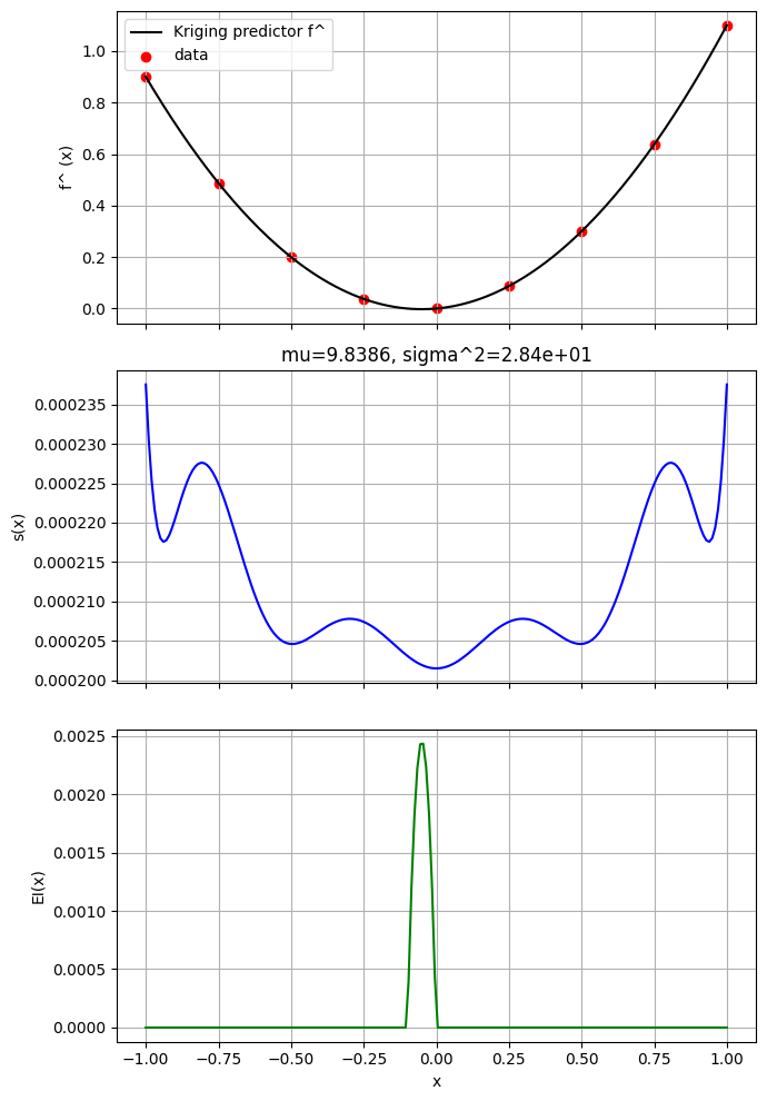
24.12 Kriging 1D demo: 3bc, 3c3^2, s(x), and EI (Forrester et al., 2008, Ch. 2/3/6)

This notebook fits the provided Kriging implementation to a 1D function and visualizes:

• The predictor f^ (x)
• The estimated mean 3bc and variance 3c3^2 from the concentrated likelihood
• The predictive standard deviation s(x)
• The Expected Improvement (EI) curve (for minimization)

%matplotlib inline
import numpy as np
import matplotlib.pyplot as plt
from spotpython.surrogate.kriging import Kriging

# 1D training data (noisy-free quadratic)
rng = np.random.default_rng(0)
X_train = np.linspace(-1.0, 1.0, 9).reshape(-1, 1)
y_train = (X_train[:, 0]**2 + 0.1*X_train[:, 0]).astype(float)

# Fit Kriging (regression with nugget optimization)
model = Kriging(method="regression", var_type=["num"], seed=124)
model.fit(X_train, y_train)
print("theta(log10):", model.theta)
print("Lambda(log10):", model.Lambda)

theta(log10): [-1.14274728]
Lambda(log10): [-8.99954829]

# Compute \u03bc and \u03c3^2 as in likelihood() (Forrester Ch. 3)
y = model.y_.flatten()
n = model.X_.shape[0]
one = np.ones(n)
U = model.U_

temp_y = np.linalg.solve(U, y)
temp_1 = np.linalg.solve(U, one)
vy = np.linalg.solve(U.T, temp_y)
v1 = np.linalg.solve(U.T, temp_1)
mu = (one @ vy) / (one @ v1)
resid = y - one * mu
tresid = np.linalg.solve(U, resid)
tresid = np.linalg.solve(U.T, tresid)
sigma2 = (resid @ tresid) / n
print(f"mu: {mu:.6f}, sigma^2: {sigma2:.6e}")

mu: 9.838641, sigma^2: 2.836785e+01

# Prediction grid
X_grid = np.linspace(X_train.min(), X_train.max(), 200).reshape(-1, 1)

# Predict f^(x) and s(x)
y_pred, s_pred = model.predict(X_grid, return_std=True)

# EI: model.predict(..., return_val="all") returns (y, s, -log10(EI))
y_all, s_all, neg_log10_ei = model.predict(X_grid, return_val="all")
EI = 10.0 ** (-neg_log10_ei)

fig, axs = plt.subplots(3, 1, figsize=(7, 10), sharex=True)

# 1) Predictor with data
axs[0].plot(X_grid[:, 0], y_pred, 'k', label='Kriging predictor f^')
axs[0].scatter(X_train[:, 0], y_train, c='r', label='data')
axs[0].set_ylabel('f^ (x)')
axs[0].grid(True)
axs[0].legend(loc='best')

# 2) Predictive standard deviation
axs[1].plot(X_grid[:, 0], s_pred, 'b')
axs[1].set_ylabel('s(x)')
axs[1].grid(True)
axs[1].set_title(f"mu={mu:.4f}, sigma^2={sigma2:.2e}")

# 3) Expected Improvement (minimization)
axs[2].plot(X_grid[:, 0], EI, 'g')
axs[2].set_xlabel('x')
axs[2].set_ylabel('EI(x)')
axs[2].grid(True)

plt.tight_layout()
plt.show()