import torch
import numpy as np
import torch.nn as nn
import torch.optim as optim
import torch.utils.data as thdat
import functools
import matplotlib.pyplot as plt
import seaborn as sns

sns.set_theme()
torch.manual_seed(42)

DEVICE = torch.device("cuda" if torch.cuda.is_available() else "cpu")

# boundaries for the frequency range
a = 0
b = 50052 Physics Informed Neural Networks
52.1 PINNs
52.2 Generation and Visualization of the Training Data and the Ground Truth (Function)
- Definition of the (unknown) differential equation:
def ode(frequency, loc, sigma, R):
    """Computes the amplitude. Defining equation, used
    to generate data and train models.
    The equation itself is not known to the model.

    Args:
        frequency: (N,) array-like
        loc: float
        sigma: float
        R: float

    Returns:
        (N,) array-like

    Examples:
        >>> ode(0, 25, 100, 0.005)
        100.0
    """
    A = np.exp(-R * (frequency - loc)**2/sigma**2)
return A- Setting the parameters for the ode
np.random.seed(10)
loc = 250
sigma = 100
R = 0.5- Generating the data
frequencies = np.linspace(a, b, 1000)
eq = functools.partial(ode, loc=loc, sigma=sigma, R=R)
amplitudes = eq(frequencies)- Now we have the ground truth for the full frequency range and can take a look at the first 10 values:
import pandas as pd
df = pd.DataFrame({'Frequency': frequencies[:10], 'Amplitude': amplitudes[:10]})
print(df)
Frequency Amplitude
0 0.000000 0.043937
1 0.500501 0.044490
2 1.001001 0.045048
3 1.501502 0.045612
4 2.002002 0.046183
5 2.502503 0.046759
6 3.003003 0.047341
7 3.503504 0.047929
8 4.004004 0.048524
9 4.504505 0.049124- We generate the training data as a subset of the full frequency range and add some noise:
t = np.linspace(a, 2*b/3, 10)
A = eq(t) + 0.2 * np.random.randn(10)- Plot of the training data and the ground truth:
plt.plot(frequencies, amplitudes)
plt.plot(t, A, 'o')
plt.legend(['Equation (ground truth)', 'Training data'])
plt.ylabel('Amplitude')
plt.xlabel('Frequency')
Text(0.5, 0, 'Frequency')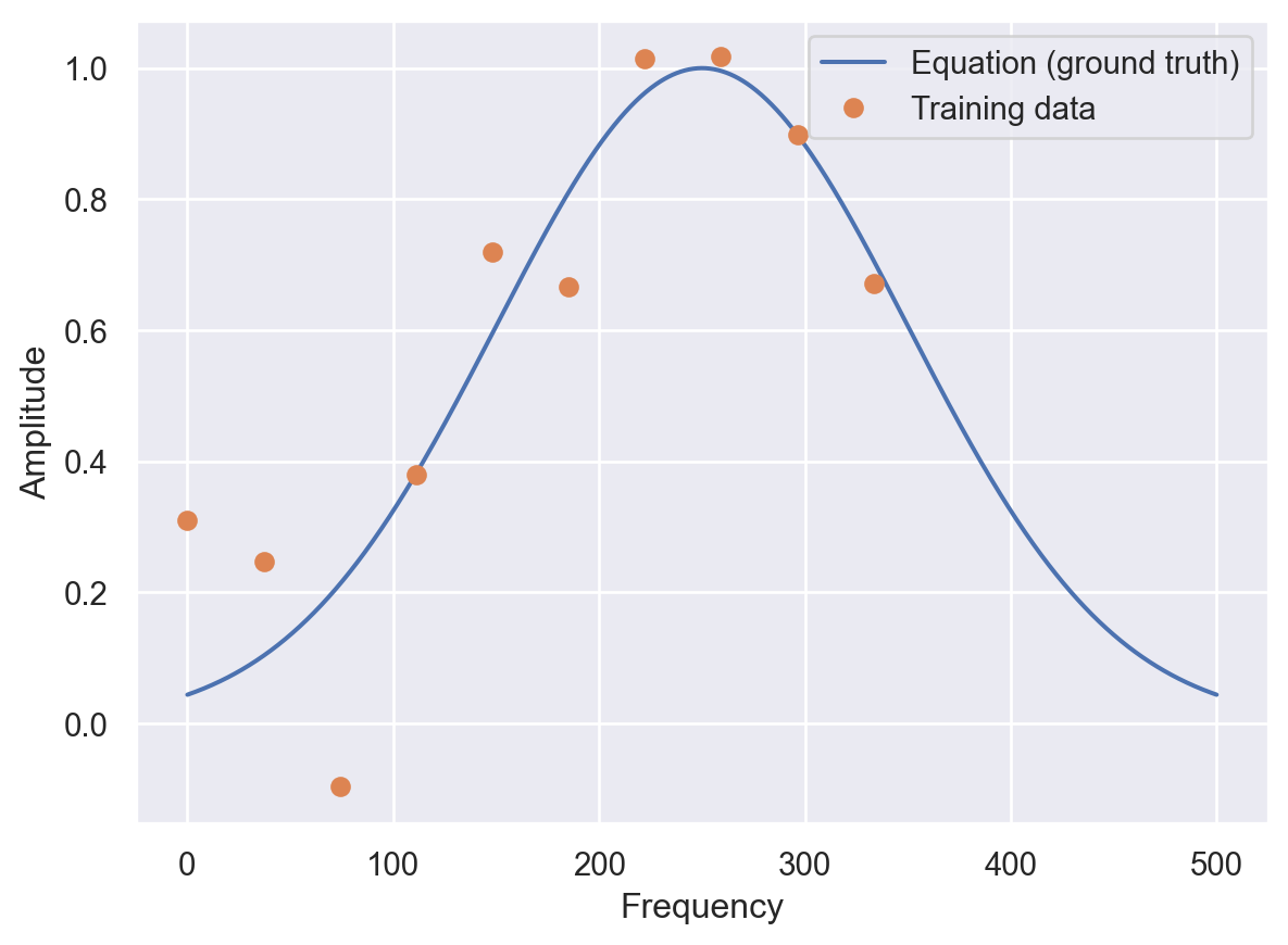
52.3 Gradient With Autograd
def grad(outputs, inputs):
    """Computes the partial derivative of
    an output with respect to an input.

    Args:
        outputs: (N, 1) tensor
        inputs: (N, D) tensor

    Returns:
        (N, D) tensor

    Examples:
        >>> x = torch.tensor([1.0, 2.0, 3.0], requires_grad=True)
        >>> y = x**2
        >>> grad(y, x)
        tensor([2., 4., 6.])
    """
    return torch.autograd.grad(
        outputs, inputs, grad_outputs=torch.ones_like(outputs), create_graph=True
)- Autograd example:
x = torch.tensor([1.0, 2.0, 3.0], requires_grad=True)
y = x**2
grad(y, x)
(tensor([2., 4., 6.], grad_fn=<MulBackward0>),)52.4 Network
def numpy2torch(x):
    """Converts a numpy array to a pytorch tensor.

    Args:
        x: (N, D) array-like

    Returns:
        (N, D) tensor

    Examples:
        >>> numpy2torch(np.array([1,2,3]))
        tensor([1., 2., 3.])
    """
    n_samples = len(x)
    return torch.from_numpy(x).to(torch.float).to(DEVICE).reshape(n_samples, -1)
class Net(nn.Module):
def __init__(
self,
input_dim,
output_dim,
n_units=100,
epochs=1000,
loss=nn.MSELoss(),
lr=1e-3,
loss2=None,
loss2_weight=0.1,
) -> None:
super().__init__()
self.epochs = epochs
self.loss = loss
self.loss2 = loss2
self.loss2_weight = loss2_weight
self.lr = lr
self.n_units = n_units
self.layers = nn.Sequential(
nn.Linear(input_dim, self.n_units),
nn.ReLU(),
nn.Linear(self.n_units, self.n_units),
nn.ReLU(),
nn.Linear(self.n_units, self.n_units),
nn.ReLU(),
nn.Linear(self.n_units, self.n_units),
nn.ReLU(),
)
self.out = nn.Linear(self.n_units, output_dim)
def forward(self, x):
h = self.layers(x)
out = self.out(h)
return out
def fit(self, X, y):
Xt = numpy2torch(X)
yt = numpy2torch(y)
optimiser = optim.Adam(self.parameters(), lr=self.lr)
self.train()
losses = []
for ep in range(self.epochs):
optimiser.zero_grad()
outputs = self.forward(Xt)
loss = self.loss(yt, outputs)
if self.loss2:
loss += self.loss2_weight + self.loss2_weight * self.loss2(self)
loss.backward()
optimiser.step()
losses.append(loss.item())
if ep % int(self.epochs / 10) == 0:
print(f"Epoch {ep}/{self.epochs}, loss: {losses[-1]:.2f}")
return losses
def predict(self, X):
self.eval()
out = self.forward(numpy2torch(X))
return out.detach().cpu().numpy()- Extended network for parameter estimation of parameter
r:
class PINNParam(Net):
    def __init__(
        self,
        input_dim,
        output_dim,
        n_units=100,
        epochs=1000,
        loss=nn.MSELoss(),
        lr=0.001,
        loss2=None,
        loss2_weight=0.1,
    ) -> None:
        super().__init__(
            input_dim, output_dim, n_units, epochs, loss, lr, loss2, loss2_weight
        )

        self.r = nn.Parameter(data=torch.tensor([1.]))
        self.sigma = nn.Parameter(data=torch.tensor([100.]))
        self.loc = nn.Parameter(data=torch.tensor([100.]))
52.5 Basic Neutral Network
- Network without regularization:
net = Net(1,1, loss2=None, epochs=2000, lr=1e-5).to(DEVICE)

losses = net.fit(t, A)

plt.plot(losses)
plt.yscale('log')
Epoch 0/2000, loss: 6.59
Epoch 200/2000, loss: 0.06
Epoch 400/2000, loss: 0.05
Epoch 600/2000, loss: 0.05
Epoch 800/2000, loss: 0.05
Epoch 1000/2000, loss: 0.05
Epoch 1200/2000, loss: 0.05
Epoch 1400/2000, loss: 0.05
Epoch 1600/2000, loss: 0.05
Epoch 1800/2000, loss: 0.05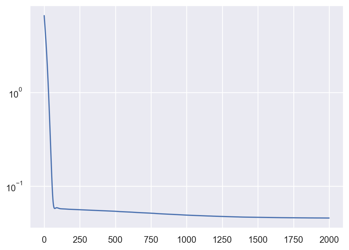
- Adding L2 regularization:
def l2_reg(model: torch.nn.Module):
    """L2 regularization for the model parameters.

    Args:
        model: torch.nn.Module

    Returns:
        torch.Tensor

    Examples:
        >>> l2_reg(Net(1,1))
        tensor(0.0001, grad_fn=<SumBackward0>)
    """
    return torch.sum(sum([p.pow(2.) for p in model.parameters()]))
netreg = Net(1,1, loss2=l2_reg, epochs=20000, lr=1e-5, loss2_weight=.1).to(DEVICE)
losses = netreg.fit(t, A)
plt.plot(losses)
plt.yscale('log')Epoch 0/20000, loss: 662.07
Epoch 2000/20000, loss: 612.81
Epoch 4000/20000, loss: 571.31
Epoch 6000/20000, loss: 533.74
Epoch 8000/20000, loss: 499.32
Epoch 10000/20000, loss: 467.44
Epoch 12000/20000, loss: 437.53
Epoch 14000/20000, loss: 409.15
Epoch 16000/20000, loss: 382.10
Epoch 18000/20000, loss: 356.29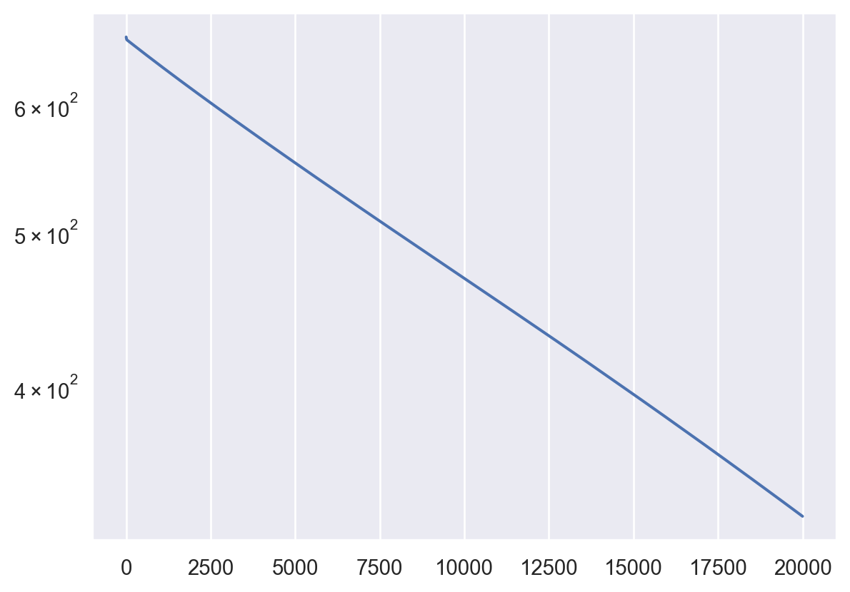
predsreg = netreg.predict(frequencies)
preds = net.predict(frequencies)
plt.plot(frequencies, amplitudes, alpha=0.8)
plt.plot(t, A, 'o')
plt.plot(frequencies, preds, alpha=0.8)
plt.plot(frequencies, predsreg, alpha=0.8)

plt.legend(labels=['Equation','Training data', 'Network', 'L2 Regularization Network'])
plt.ylabel('Amplitude')
plt.xlabel('Frequency')
Text(0.5, 0, 'Frequency')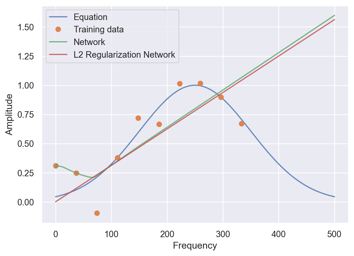
52.6 PINNs
- Calculate the physics-informed loss (similar to the L2 regularization):
def physics_loss(model: torch.nn.Module):
    """Computes the physics-informed loss for the model.

    Args:
        model: torch.nn.Module

    Returns:
        torch.Tensor

    Examples:
        >>> physics_loss(Net(1,1))
        tensor(0.0001, grad_fn=<MeanBackward0>)
    """
    ts = torch.linspace(a, b, steps=1000).view(-1,1).requires_grad_(True).to(DEVICE)
    amplitudes = model(ts)
    dT = grad(amplitudes, ts)[0]
    ode = -2*R*(ts-loc)/ sigma**2 * amplitudes - dT
return torch.mean(ode**2)- Train the network with the physics-informed loss and plot the training error:
net_pinn = Net(1,1, loss2=physics_loss, epochs=2000, loss2_weight=1, lr=1e-5).to(DEVICE)
losses = net_pinn.fit(t, A)
plt.plot(losses)
plt.yscale('log')
Epoch 0/2000, loss: 12.23
Epoch 200/2000, loss: 1.05
Epoch 400/2000, loss: 1.05
Epoch 600/2000, loss: 1.05
Epoch 800/2000, loss: 1.05
Epoch 1000/2000, loss: 1.05
Epoch 1200/2000, loss: 1.05
Epoch 1400/2000, loss: 1.05
Epoch 1600/2000, loss: 1.05
Epoch 1800/2000, loss: 1.05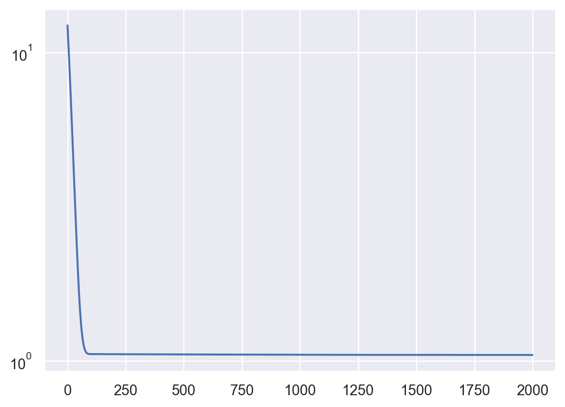
- Predict the amplitude and plot the results:
preds_pinn = net_pinn.predict(frequencies)
plt.plot(frequencies, amplitudes, alpha=0.8)
plt.plot(t, A, 'o')
plt.plot(frequencies, preds, alpha=0.8)
plt.plot(frequencies, predsreg, alpha=0.8)
plt.plot(frequencies, preds_pinn, alpha=0.8)
plt.legend(labels=['Equation','Training data', 'NN', "R2", 'PINN'])
plt.ylabel('Amplitude')
plt.xlabel('Frequency')
Text(0.5, 0, 'Frequency')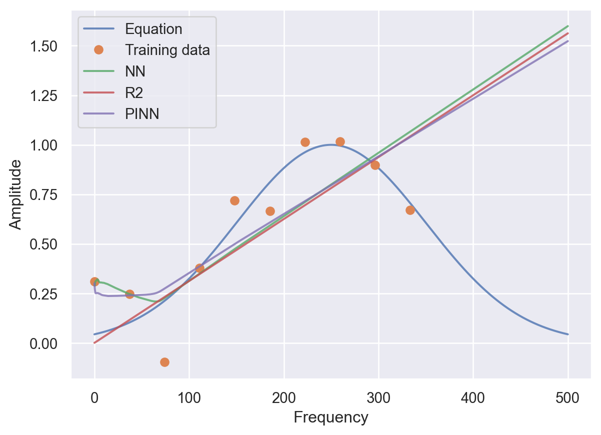
52.6.1 PINNs: Parameter Estimation
def physics_loss_estimation(model: torch.nn.Module):
    ts = torch.linspace(a, b, steps=1000,).view(-1,1).requires_grad_(True).to(DEVICE)
    amplitudes = model(ts)
    dT = grad(amplitudes, ts)[0]
    ode = -2*model.r*(ts-model.loc)/ (model.sigma)**2 * amplitudes - dT
    return torch.mean(ode**2)
pinn_param = PINNParam(1, 1, loss2=physics_loss_estimation, loss2_weight=1, epochs=4000, lr= 5e-6).to(DEVICE)
losses = pinn_param.fit(t, A)
plt.plot(losses)
plt.yscale('log')Epoch 0/4000, loss: 15.06
Epoch 400/4000, loss: 1.06
Epoch 800/4000, loss: 1.06
Epoch 1200/4000, loss: 1.06
Epoch 1600/4000, loss: 1.05
Epoch 2000/4000, loss: 1.05
Epoch 2400/4000, loss: 1.05
Epoch 2800/4000, loss: 1.05
Epoch 3200/4000, loss: 1.05
Epoch 3600/4000, loss: 1.05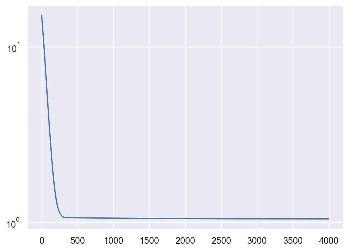
preds_disc = pinn_param.predict(frequencies)
print(f"Estimated r: {pinn_param.r}")
print(f"Estimated sigma: {pinn_param.sigma}")
print(f"Estimated loc: {pinn_param.loc}")
Estimated r: Parameter containing:
tensor([0.9893], requires_grad=True)
Estimated sigma: Parameter containing:
tensor([100.0067], requires_grad=True)
Estimated loc: Parameter containing:
tensor([100.0065], requires_grad=True)plt.plot(frequencies, amplitudes, alpha=0.8)
plt.plot(t, A, 'o')
plt.plot(frequencies, preds_disc, alpha=0.8)
plt.legend(labels=['Equation','Training data', 'estimation PINN'])
plt.ylabel('Amplitude')
plt.xlabel('Frequency')Text(0.5, 0, 'Frequency')
plt.plot(frequencies, amplitudes, alpha=0.8)
plt.plot(t, A, 'o')
plt.plot(frequencies, preds, alpha=0.8)
plt.plot(frequencies, predsreg, alpha=0.8)
plt.plot(frequencies, preds_pinn, alpha=0.8)
plt.plot(frequencies, preds_disc, alpha=0.8)
plt.legend(labels=['Equation','Training data', 'NN', "R2", 'PINN', 'paramPINN'])
plt.ylabel('Amplitude')
plt.xlabel('Frequency')
Text(0.5, 0, 'Frequency')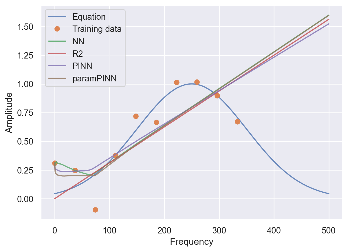
plt.plot(frequencies, amplitudes, alpha=0.8)
plt.plot(t, A, 'o')
plt.plot(frequencies, preds, alpha=0.8)
plt.plot(frequencies, predsreg, alpha=0.8)
plt.plot(frequencies, preds_disc, alpha=0.8)
plt.legend(labels=['Equation','Training data', 'NN', "R2", 'paramPINN'])
plt.ylabel('Amplitude')
plt.xlabel('Frequency')
Text(0.5, 0, 'Frequency')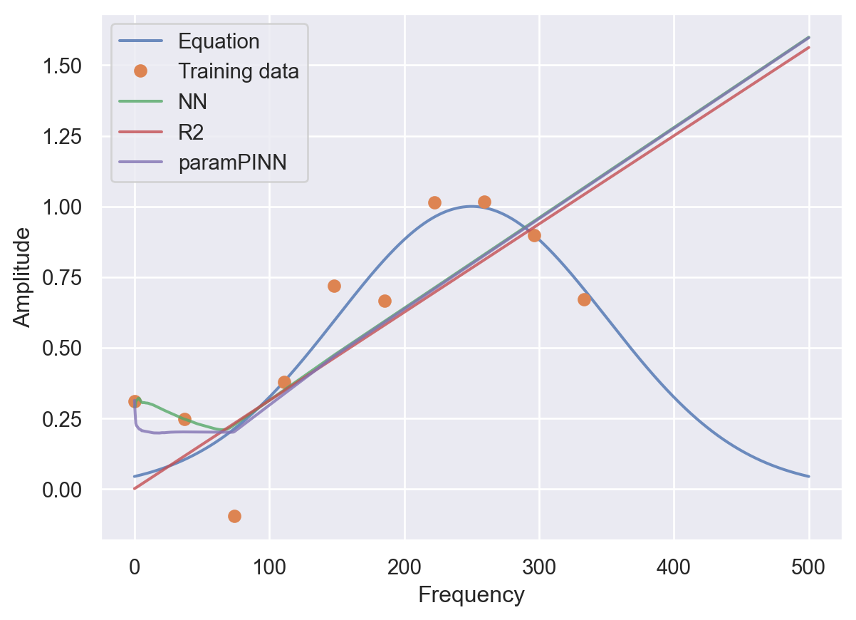
plt.plot(frequencies, amplitudes, alpha=0.8)
plt.plot(t, A, 'o')
plt.plot(frequencies, preds, alpha=0.8)
plt.plot(frequencies, predsreg, alpha=0.8)
plt.plot(frequencies, preds_disc, alpha=0.8)
plt.legend(labels=['Grundwahrheit','Trainingsdaten', 'NN', "NN+R2", 'PINN'])
plt.ylabel('Amplitude')
plt.xlabel('Frequenz')
# save the plot as a pdf
plt.savefig('pinns.pdf')
plt.savefig('pinns.png')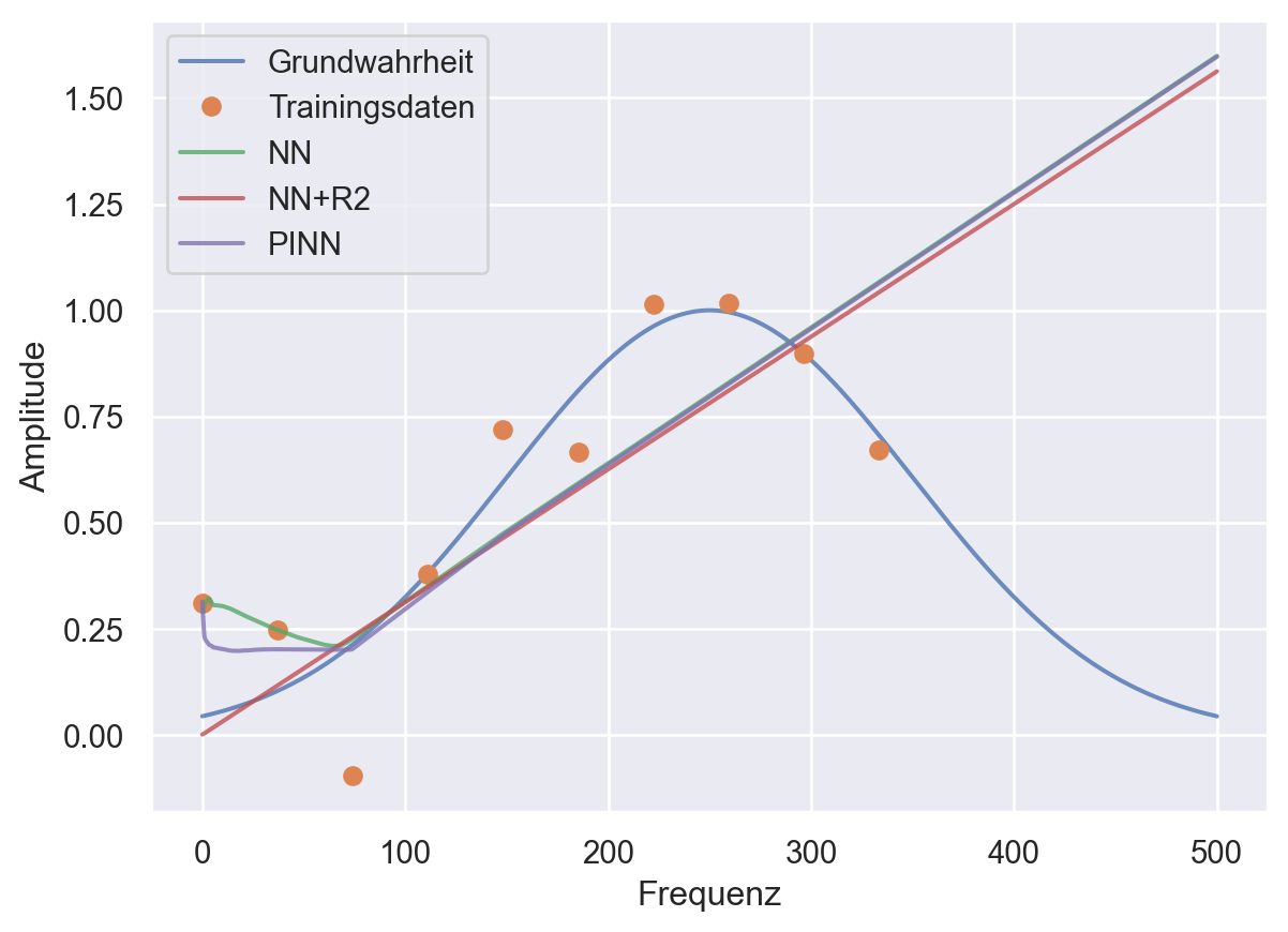
52.7 Summary
- Results strongly depend on the parametrization(s)
- PINN parameter estimation not robust
- Hyperparameter tuning is crucial
- Use SPOT before further analysis is done