import numpy as np
from math import inf
from spotpython.fun.objectivefunctions import Analytical
from spotpython.spot import Spot
import matplotlib.pyplot as plt
from spotpython.utils.init import fun_control_init, get_spot_tensorboard_path
from spotpython.utils.init import fun_control_init, design_control_init, surrogate_control_init
PREFIX = "14"20 Optimal Computational Budget Allocation in spotpython
This chapter demonstrates how noisy functions can be handled spotpython:
- First, Optimal Computational Budget Allocation (OCBA) is introduced in Chapter 20.
- Then, the nugget effect is explained in Section 20.3.
Citation
If this document has been useful to you and you wish to cite it in a scientific publication, please refer to the following paper, which can be found on arXiv: https://arxiv.org/abs/2307.10262.
@ARTICLE{bart23iArXiv,
      author = {{Bartz-Beielstein}, Thomas},
      title = "{Hyperparameter Tuning Cookbook:
          A guide for scikit-learn, PyTorch, river, and spotpython}",
     journal = {arXiv e-prints},
    keywords = {Computer Science - Machine Learning,
      Computer Science - Artificial Intelligence, 90C26, I.2.6, G.1.6},
         year = 2023,
        month = jul,
          eid = {arXiv:2307.10262},
          doi = {10.48550/arXiv.2307.10262},
archivePrefix = {arXiv},
       eprint = {2307.10262},
 primaryClass = {cs.LG}
}
20.1 Example: spotpython, OCBA, and the Noisy Sphere Function
20.1.1 The Objective Function: Noisy Sphere
The spotpython package provides several classes of objective functions. We will use an analytical objective function with noise, i.e., a function that can be described by a (closed) formula: \[f(x) = x^2 + \epsilon\]
Since sigma is set to 0.1, noise is added to the function:
fun = Analytical().fun_sphere
fun_control = fun_control_init(
    PREFIX=PREFIX,
    sigma=0.1)
A plot (Figure 20.1) illustrates the noise:
x = np.linspace(-1,1,100).reshape(-1,1)
y = fun(x, fun_control=fun_control)
plt.figure()
plt.plot(x,y, "k")
plt.show()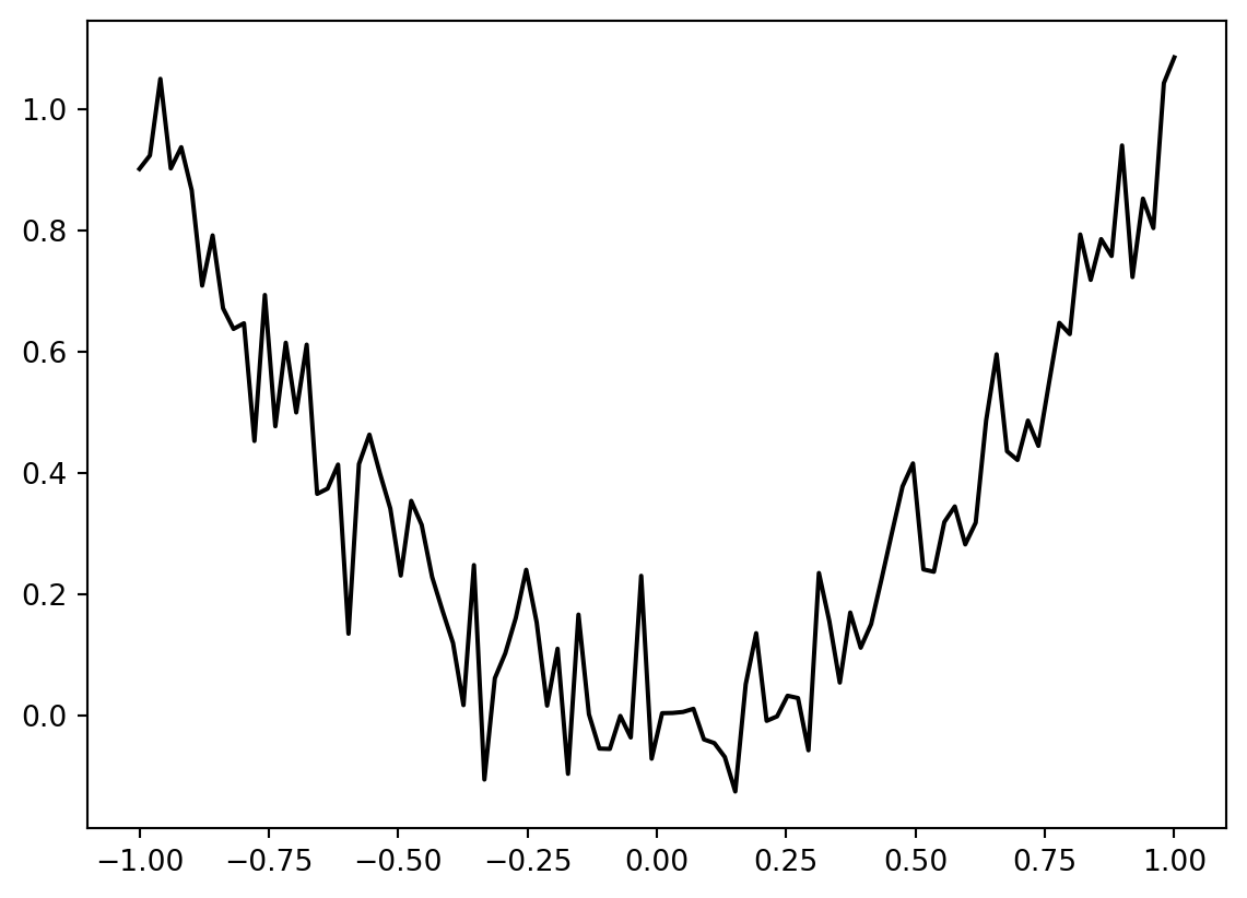
NoteNoise Handling in
spotpython
spotpython has several options to cope with noisy functions:
fun_repeatsis set to a value larger than 1, e.g., 2, which means every function evaluation during the search on the surrogate is repeated twice. The mean of the two evaluations is used as the function value.init size(of thedesign_controldictionary) is set to a value larger than 1 (here: 2).ocba_deltais set to a value larger than 1 (here: 2). This means that the OCBA algorithm is used to allocate the computational budget optimally.- Using a nugget term in the surrogate model. This is done by setting
method="regression"in thesurrogate_controldictionary. An example is given in Section 20.3.
20.2 Using Optimal Computational Budget Allocation (OCBA)
The Optimal Computational Budget Allocation (OCBA) algorithm is a powerful tool for efficiently distributing computational resources (Chen 2010). It is specifically designed to maximize the Probability of Correct Selection (PCS) while minimizing computational costs. By strategically allocating more simulation effort to design alternatives that are either more challenging to evaluate or more likely to yield optimal results, OCBA ensures an efficient use of resources. This approach enables researchers and decision-makers to achieve accurate outcomes more quickly and with fewer computational demands, making it an invaluable method for simulation optimization.
The OCBA algorithm is implemented in spotpython and can be used by setting ocba_delta to a value larger than 0. The source code is available in the spotpython package, see [DOC]. See also Bartz-Beielstein et al. (2011).
Example 20.1 To reproduce the example from p.49 in Chen (2010), the following spotpython code can be used:
import numpy as np
from spotpython.budget.ocba import get_ocba
mean_y = np.array([1,2,3,4,5])
var_y = np.array([1,1,9,9,4])
get_ocba(mean_y, var_y, 50)
array([11, 9, 19, 9, 2])20.2.1 The Noisy Sphere
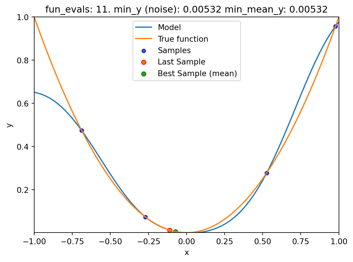
We will demonstrate the OCBA algorithm on the noisy sphere function defined in Section 20.1.1. The OCBA algorithm is used to allocate the computational budget optimally. This means that the function evaluations are repeated several times, and the best function value is used for the next iteration.
NoteVisualizing the Search of the OCBA Algorithm
- The
show_modelsparameter in thefun_controldictionary is set toTrue. This means that the surrogate model is shown during the search. - To keep the visualization simple, only the ground truth and the surrogate model are shown. The surrogate model is shown in blue, and the ground truth is shown in orange. The noisy function was shown in Figure 20.1.
spot_1_noisy = Spot(fun=fun,
                   fun_control=fun_control_init(
                   lower = np.array([-1]),
                   upper = np.array([1]),
                   fun_evals = 20,
                   fun_repeats = 1,
                   noise = True,
                   tolerance_x=0.0,
                   ocba_delta = 2,
                   show_models=True),
                   design_control=design_control_init(init_size=5, repeats=2),
                   surrogate_control=surrogate_control_init(method="regression"))
spot_1_noisy.run()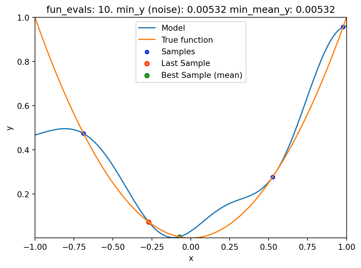
spotpython tuning: 0.005320352324811128 [######----] 55.00%. Success rate: 0.00% 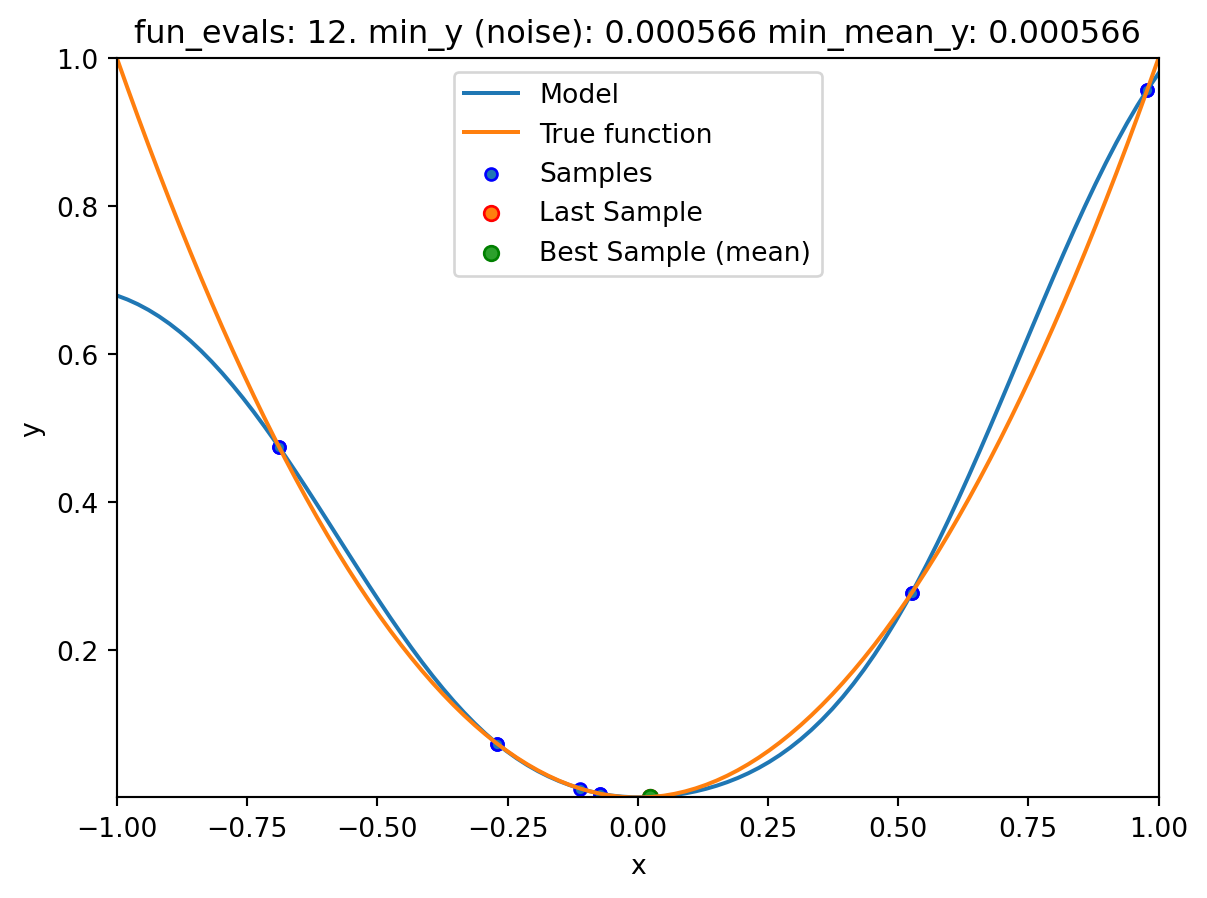
spotpython tuning: 0.0004783786250623159 [######----] 60.00%. Success rate: 50.00% 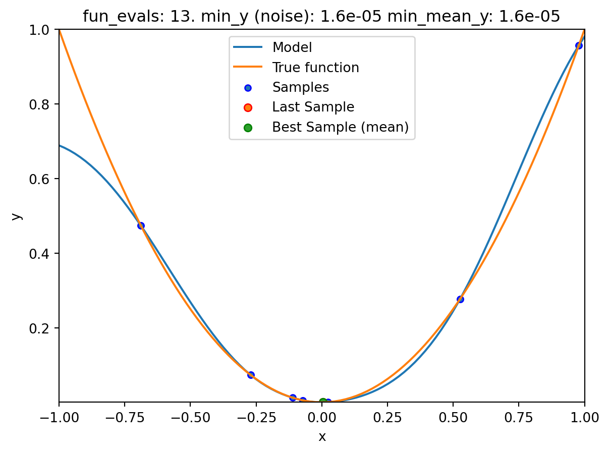
spotpython tuning: 1.1021305166700617e-07 [######----] 65.00%. Success rate: 66.67% 
spotpython tuning: 1.1021305166700617e-07 [#######---] 70.00%. Success rate: 50.00% 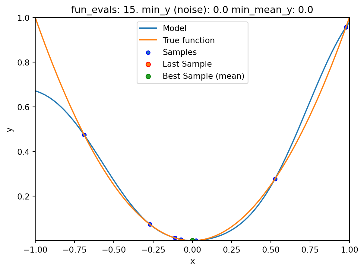
spotpython tuning: 1.2330075308902535e-11 [########--] 75.00%. Success rate: 60.00% 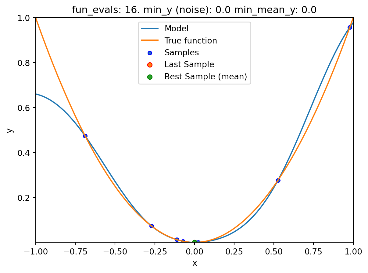
spotpython tuning: 1.1089814189632306e-11 [########--] 80.00%. Success rate: 66.67% 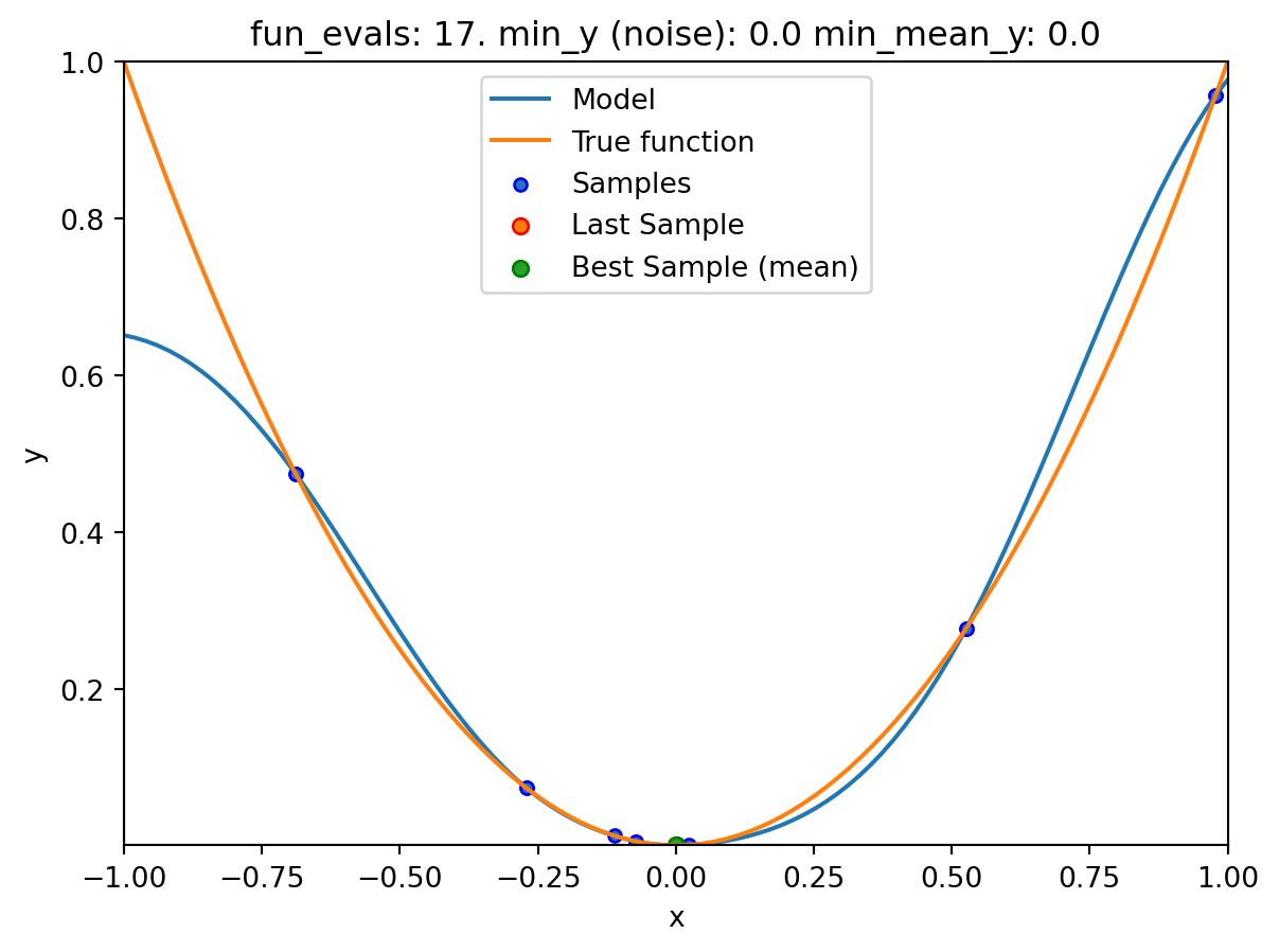
spotpython tuning: 7.071108734979218e-13 [########--] 85.00%. Success rate: 71.43% 
spotpython tuning: 7.071108734979218e-13 [#########-] 90.00%. Success rate: 62.50% 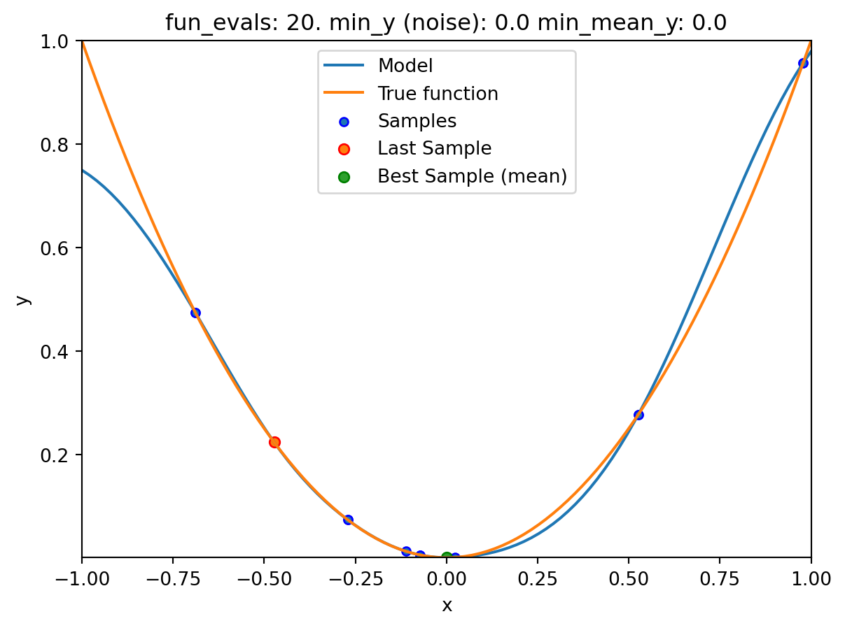
spotpython tuning: 7.071108734979218e-13 [##########] 95.00%. Success rate: 55.56% 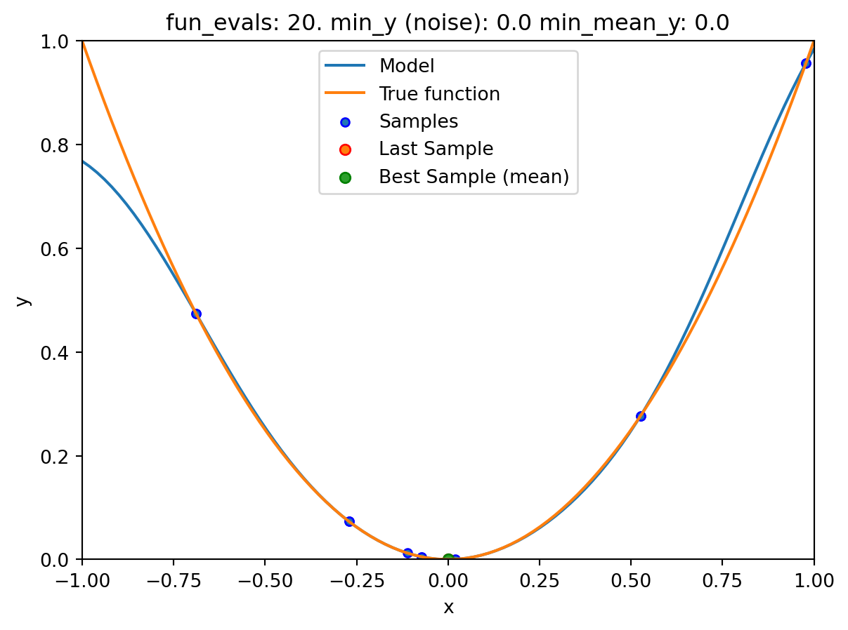
spotpython tuning: 7.071108734979218e-13 [##########] 100.00%. Success rate: 50.00% Done...

Experiment saved to 000_res.pkl
20.2.2 Print the Results
spot_1_noisy.print_results()min y: 7.071108734979218e-13
min mean y: 7.071108734979218e-13
x0: -8.408988485530955e-07[['x0', np.float64(-8.408988485530955e-07)]]spot_1_noisy.plot_progress(log_y=True)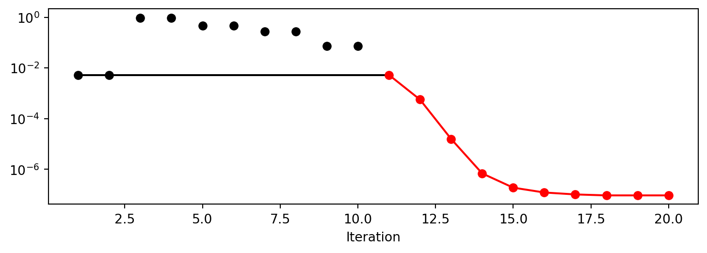
20.3 Noise and Surrogates: The Nugget Effect
In the previous example, we have seen that the fun_repeats parameter can be used to repeat function evaluations. This is useful when the function is noisy. However, it is not always possible to repeat function evaluations, e.g., when the function is expensive to evaluate. In this case, we can use a surrogate model with a nugget term. The nugget term is a small value that is added to the diagonal of the covariance matrix. This allows the surrogate model to fit the data better, even if the data is noisy. The nugget term is added, if method="regression" is set in the surrogate_control dictionary.
20.3.1 The Noisy Sphere
20.3.1.1 The Data
We prepare some data first:
import numpy as np
import spotpython
from spotpython.fun.objectivefunctions import Analytical
from spotpython.spot import Spot
from spotpython.design.spacefilling import SpaceFilling
from spotpython.surrogate.kriging import Kriging
import matplotlib.pyplot as plt

gen = SpaceFilling(1)
rng = np.random.RandomState(1)
lower = np.array([-10])
upper = np.array([10])
fun = Analytical().fun_sphere
fun_control = fun_control_init(
    sigma=2,
    seed=125)
X = gen.scipy_lhd(10, lower=lower, upper = upper)
y = fun(X, fun_control=fun_control)
X_train = X.reshape(-1,1)
y_train = y
A surrogate without nugget is fitted to these data:
S = Kriging(name='kriging',
            seed=123,
            log_level=50,
            isotropic=True,
            method="interpolation")
S.fit(X_train, y_train)

X_axis = np.linspace(start=-13, stop=13, num=1000).reshape(-1, 1)
mean_prediction, std_prediction, ei = S.predict(X_axis, return_val="all")

plt.scatter(X_train, y_train, label="Observations")
plt.plot(X_axis, mean_prediction, label="mue")
plt.legend()
plt.xlabel("$x$")
plt.ylabel("$f(x)$")
_ = plt.title("Sphere: Gaussian process regression on noisy dataset")
In comparison to the surrogate without nugget, we fit a surrogate with nugget to the data:
S_nug = Kriging(name='kriging',
            seed=123,
            log_level=50,
            isotropic=True,
            method="regression")
S_nug.fit(X_train, y_train)
X_axis = np.linspace(start=-13, stop=13, num=1000).reshape(-1, 1)
mean_prediction, std_prediction, ei = S_nug.predict(X_axis, return_val="all")
plt.scatter(X_train, y_train, label="Observations")
plt.plot(X_axis, mean_prediction, label="mue")
plt.legend()
plt.xlabel("$x$")
plt.ylabel("$f(x)$")
_ = plt.title("Sphere: Gaussian process regression with nugget on noisy dataset")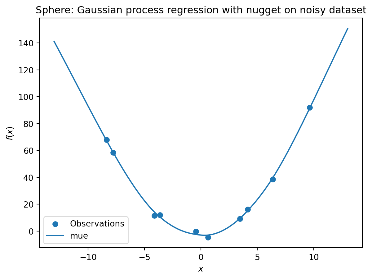
The value of the nugget term can be extracted from the model as follows:
S.Lambda10**S_nug.Lambdaarray([7.80803702e-05])We see:
- the first model
Shas no nugget, - whereas the second model has a nugget value (
Lambda) larger than zero.
20.4 Exercises
20.4.1 Noisy fun_cubed
Analyse the effect of noise on the fun_cubed function with the following settings:
fun = Analytical().fun_cubed
fun_control = fun_control_init(
    sigma=10,
    seed=123)
lower = np.array([-10])
upper = np.array([10])
20.4.2 fun_runge
Analyse the effect of noise on the fun_runge function with the following settings:
lower = np.array([-10])
upper = np.array([10])
fun = Analytical().fun_runge
fun_control = fun_control_init(
    sigma=0.25,
    seed=123)
20.4.3 fun_forrester
Analyse the effect of noise on the fun_forrester function with the following settings:
lower = np.array([0])
upper = np.array([1])
fun = Analytical().fun_forrester
fun_control = {"sigma": 5,
               "seed": 123}
20.4.4 fun_xsin
Analyse the effect of noise on the fun_xsin function with the following settings:
lower = np.array([-1.])
upper = np.array([1.])
fun = Analytical().fun_xsin
fun_control = fun_control_init(
    sigma=0.5,
    seed=123)
20.5 Jupyter Notebook
Note
- The Jupyter-Notebook of this chapter is available on GitHub in the Hyperparameter-Tuning-Cookbook Repository