7  Introduction to spotpython

Surrogate model based optimization methods are common approaches in simulation and optimization. SPOT was developed because there is a great need for sound statistical analysis of simulation and optimization algorithms. SPOT includes methods for tuning based on classical regression and analysis of variance techniques. It presents tree-based models such as classification and regression trees and random forests as well as Bayesian optimization (Gaussian process models, also known as Kriging). Combinations of different meta-modeling approaches are possible. SPOT comes with a sophisticated surrogate model based optimization method, that can handle discrete and continuous inputs. Furthermore, any model implemented in scikit-learn can be used out-of-the-box as a surrogate in spotpython.

SPOT implements key techniques such as exploratory fitness landscape analysis and sensitivity analysis. It can be used to understand the performance of various algorithms, while simultaneously giving insights into their algorithmic behavior.

The spot loop consists of the following steps:

1. Init: Build initial design \(X\)
2. Evaluate initial design on real objective \(f\): \(y = f(X)\)
3. Build surrogate: \(S = S(X,y)\)
4. Optimize on surrogate: \(X_0 = \text{optimize}(S)\)
5. Evaluate on real objective: \(y_0 = f(X_0)\)
6. Impute (Infill) new points: \(X = X \cup X_0\), \(y = y \cup y_0\).
7. Goto 3.

7.1 Advantages of the spotpython approach

• Neural networks and many ML algorithms are non-deterministic, so results are noisy (i.e., depend on the the initialization of the weights). Enhanced noise handling strategies, OCBA (description from HPT-book).

• Optimal Computational Budget Allocation (OCBA) is a very efficient solution to solve the “general ranking and selection problem” if the objective function is noisy. It allocates function evaluations in an uneven manner to identify the best solutions and to reduce the total optimization costs. [Chen10a, Bart11b] Given a total number of optimization samples \(N\) to be allocated to \(k\) competing solutions whose performance is depicted by random variables with means \(\bar{y}_i\) (\(i=1, 2, \ldots, k\)), and finite variances \(\sigma_i^2\), respectively, as \(N \to \infty\), the can be asymptotically maximized when \[\begin{align} \frac{N_i}{N_j} & = \left( \frac{ \sigma_i / \delta_{b,i}}{\sigma_j/ \delta_{b,j}} \right)^2, i,j \in \{ 1, 2, \ldots, k\}, \text{ and } i \neq j \neq b,\\ N_b &= \sigma_b \sqrt{ \sum_{i=1, i\neq b}^k \frac{N_i^2}{\sigma_i^2} }, \end{align}\] where \(N_i\) is the number of replications allocated to solution \(i\), \(\delta_{b,i} = \bar{y}_b - \bar{y}_i\), and \(\bar{y}_b \leq \min_{i\neq b} \bar{y}_i\) Bartz-Beielstein and Friese (2011).

• Surrogate-based optimization: Better than grid search and random search (Reference to HPT-book)

• Visualization

• Importance based on the Kriging model

• Sensitivity analysis. Exploratory fitness landscape analysis. Provides XAI methods (feature importance, integrated gradients, etc.)

• Uncertainty quantification

• Flexible, modular meta-modeling handling. spotpython come with a Kriging model, which can be replaced by any model implemented in scikit-learn.

• Enhanced metric handling, especially for categorical hyperparameters (any sklearn metric can be used). Default is..

• Integration with TensorBoard: Visualization of the hyperparameter tuning process, of the training steps, the model graph. Parallel coordinates plot, scatter plot matrix, and more.

• Reproducibility. Results are stored as pickle files. The results can be loaded and visualized at any time and be transferred between different machines and operating systems.

• Handles scikit-learn models and pytorch models out-of-the-box. The user has to add a simple wrapper for passing the hyperparemeters to use a pytorch model in spotpython.

• Compatible with Lightning.

• User can add own models as plain python code.

• User can add own data sets in various formats.

• Flexible data handling and data preprocessing.

• Many examples online (hyperparameter-tuning-cookbook).

• spotpython uses a robust optimizer that can even deal with hyperparameter-settings that cause crashes of the algorithms to be tuned.

• even if the optimum is not found, HPT with spotpython prevents the user from choosing bad hyperparameters in a systematic way (design of experiments).

7.2 Disadvantages of the spotpython approach

• Time consuming
• Surrogate can be misguiding
• no parallelization implement yet

Central Idea: Evaluation of the surrogate model S is much cheaper (or / and much faster) than running the real-world experiment \(f\). We start with a small example.

7.3 Example: Spot and the Sphere Function

import numpy as np
from math import inf
from spotpython.fun.objectivefunctions import Analytical
from spotpython.utils.init import fun_control_init, design_control_init
from spotpython.hyperparameters.values import set_control_key_value
from spotpython.spot import Spot
import matplotlib.pyplot as plt

7.3.1 The Objective Function: Sphere

The spotpython package provides several classes of objective functions. We will use an analytical objective function, i.e., a function that can be described by a (closed) formula: \[ f(x) = x^2 \]

fun = Analytical().fun_sphere

We can apply the function fun to input values and plot the result:

x = np.linspace(-1,1,100).reshape(-1,1)
y = fun(x)
plt.figure()
plt.plot(x, y, "k")
plt.show()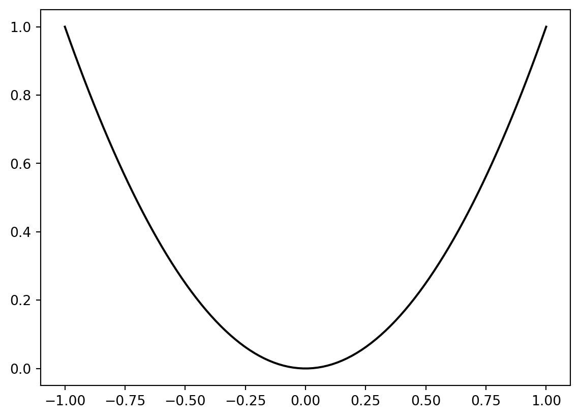

7.3.2 The Spot Method as an Optimization Algorithm Using a Surrogate Model

We initialize the fun_control dictionary. The fun_control dictionary contains the parameters for the objective function. The fun_control dictionary is passed to the Spot method.

fun_control=fun_control_init(lower = np.array([-1]),
                     upper = np.array([1]))
spot_0 = Spot(fun=fun,
                   fun_control=fun_control)
spot_0.run()

spotpython tuning: 4.960293502265715e-09 [#######---] 73.33% 
spotpython tuning: 4.959666330154525e-09 [########--] 80.00% 
spotpython tuning: 4.9571338392226926e-09 [#########-] 86.67% 
spotpython tuning: 4.9571338392226926e-09 [#########-] 93.33% 
spotpython tuning: 1.866838525968143e-10 [##########] 100.00% Done...

Experiment saved to 000_res.pkl

<spotpython.spot.spot.Spot at 0x142222ff0>

The method print_results() prints the results, i.e., the best objective function value (“min y”) and the corresponding input value (“x0”).

spot_0.print_results()

min y: 1.866838525968143e-10
x0: 1.3663229947447064e-05

[['x0', np.float64(1.3663229947447064e-05)]]

To plot the search progress, the method plot_progress() can be used. The parameter log_y is used to plot the objective function values on a logarithmic scale.

spot_0.plot_progress(log_y=True)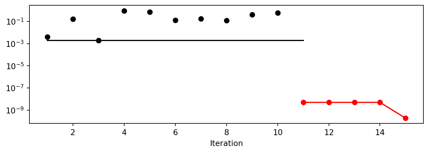

Figure 7.1: Visualization of the search progress of the Spot method. The black elements (points and line) represent the initial design, before the surrogate is build. The red elements represent the search on the surrogate.

If the dimension of the input space is one, the method plot_model() can be used to visualize the model and the underlying objective function values.

spot_0.plot_model()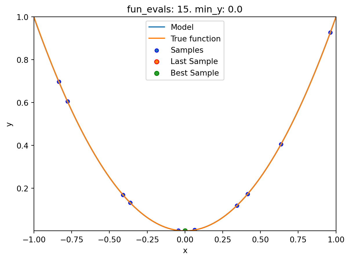

Figure 7.2: Visualization of the model and the underlying objective function values.

7.4 Spot Parameters: fun_evals, init_size and show_models

We will modify three parameters:

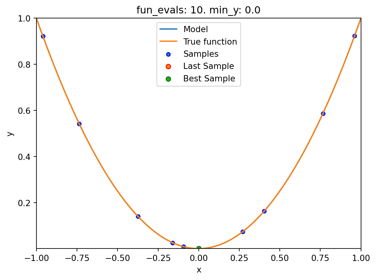
1. The number of function evaluations (fun_evals) will be set to 10 (instead of 15, which is the default value) in the fun_control dictionary.
2. The parameter show_models, which visualizes the search process for each single iteration for 1-dim functions, in the fun_control dictionary.
3. The size of the initial design (init_size) in the design_control dictionary.

The full list of the Spot parameters is shown in code reference on GitHub, see Spot.

fun_control=fun_control_init(lower = np.array([-1]),
                     upper = np.array([1]),
                     fun_evals = 10,
                     show_models = True)               
design_control = design_control_init(init_size=9)
spot_1 = Spot(fun=fun,
                   fun_control=fun_control,
                   design_control=design_control)
spot_1.run()

spotpython tuning: 9.632846333472212e-09 [##########] 100.00% Done...

Experiment saved to 000_res.pkl

7.5 Print the Results

spot_1.print_results()

min y: 9.632846333472212e-09
x0: -9.814706482351988e-05

[['x0', np.float64(-9.814706482351988e-05)]]

7.6 Show the Progress

spot_1.plot_progress()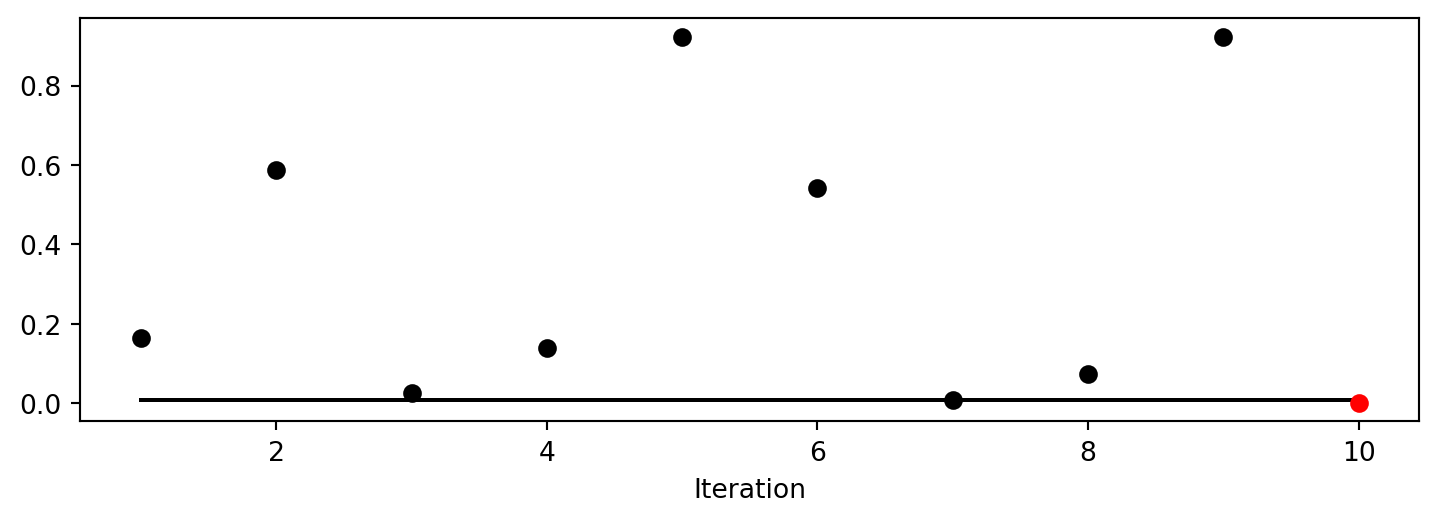

7.7 Visualizing the Optimization and Hyperparameter Tuning Process with TensorBoard

spotpython supports the visualization of the hyperparameter tuning process with TensorBoard. The following example shows how to use TensorBoard with spotpython.

First, we define an “PREFIX” to identify the hyperparameter tuning process. The PREFIX is used to create a directory for the TensorBoard files.

fun_control = fun_control_init(
    PREFIX = "01",
    lower = np.array([-1]),
    upper = np.array([2]),
    fun_evals=100,
    TENSORBOARD_CLEAN=True,
    tensorboard_log=True)
design_control = design_control_init(init_size=5)

Moving TENSORBOARD_PATH: runs/ to TENSORBOARD_PATH_OLD: runs_OLD/runs_2025_02_17_22_26_50_0
Created spot_tensorboard_path: runs/spot_logs/01_maans08_2025-02-17_22-26-50 for SummaryWriter()

Since the tensorboard_log is True, spotpython will log the optimization process in the TensorBoard files. The argument TENSORBOARD_CLEAN=True will move the TensorBoard files from the previous run to a backup folder, so that TensorBoard files from previous runs are not overwritten and a clean start in the runs folder is guaranteed.

spot_tuner = Spot(fun=fun,                   
                   fun_control=fun_control,
                   design_control=design_control)
spot_tuner.run()
spot_tuner.print_results()

spotpython tuning: 2.487613964476317e-05 [#---------] 6.00% 
spotpython tuning: 7.85064251023503e-07 [#---------] 7.00% 
spotpython tuning: 7.210284620467494e-07 [#---------] 8.00% 
spotpython tuning: 4.191441813872346e-07 [#---------] 9.00% 
spotpython tuning: 7.4015092835768465e-09 [#---------] 10.00% 
spotpython tuning: 7.4015092835768465e-09 [#---------] 11.00% 
spotpython tuning: 7.4015092835768465e-09 [#---------] 12.00% 
spotpython tuning: 7.4015092835768465e-09 [#---------] 13.00% 
spotpython tuning: 7.4015092835768465e-09 [#---------] 14.00% 
spotpython tuning: 7.4015092835768465e-09 [##--------] 15.00% 
spotpython tuning: 7.4015092835768465e-09 [##--------] 16.00% 
spotpython tuning: 7.4015092835768465e-09 [##--------] 17.00% 
spotpython tuning: 7.4015092835768465e-09 [##--------] 18.00% 
spotpython tuning: 7.4015092835768465e-09 [##--------] 19.00% 
spotpython tuning: 7.4015092835768465e-09 [##--------] 20.00% 
spotpython tuning: 6.704802934300911e-10 [##--------] 21.00% 
spotpython tuning: 6.704802934300911e-10 [##--------] 22.00% 
spotpython tuning: 6.668629799831143e-10 [##--------] 23.00% 
spotpython tuning: 6.668629799831143e-10 [##--------] 24.00% 
spotpython tuning: 6.499816856638441e-10 [##--------] 25.00% 
spotpython tuning: 6.499816856638441e-10 [###-------] 26.00% 
spotpython tuning: 6.499816856638441e-10 [###-------] 27.00% 
spotpython tuning: 6.499816856638441e-10 [###-------] 28.00% 
spotpython tuning: 6.499816856638441e-10 [###-------] 29.00% 
spotpython tuning: 6.499816856638441e-10 [###-------] 30.00% 
spotpython tuning: 6.499816856638441e-10 [###-------] 31.00% 
spotpython tuning: 6.499816856638441e-10 [###-------] 32.00% 
spotpython tuning: 6.499816856638441e-10 [###-------] 33.00% 
spotpython tuning: 6.499816856638441e-10 [###-------] 34.00% 
spotpython tuning: 6.499816856638441e-10 [####------] 35.00% 
spotpython tuning: 6.499816856638441e-10 [####------] 36.00% 
spotpython tuning: 6.499816856638441e-10 [####------] 37.00% 
spotpython tuning: 6.499816856638441e-10 [####------] 38.00% 
spotpython tuning: 6.499816856638441e-10 [####------] 39.00% 
spotpython tuning: 6.499816856638441e-10 [####------] 40.00% 
spotpython tuning: 6.499816856638441e-10 [####------] 41.00% 
spotpython tuning: 6.499816856638441e-10 [####------] 42.00% 
spotpython tuning: 6.499816856638441e-10 [####------] 43.00% 
spotpython tuning: 6.499816856638441e-10 [####------] 44.00% 
spotpython tuning: 6.499816856638441e-10 [####------] 45.00% 
spotpython tuning: 6.499816856638441e-10 [#####-----] 46.00% 
spotpython tuning: 6.499816856638441e-10 [#####-----] 47.00% 
spotpython tuning: 6.499816856638441e-10 [#####-----] 48.00% 
spotpython tuning: 6.499816856638441e-10 [#####-----] 49.00% 
spotpython tuning: 6.499816856638441e-10 [#####-----] 50.00% 
spotpython tuning: 6.499816856638441e-10 [#####-----] 51.00% 
spotpython tuning: 6.499816856638441e-10 [#####-----] 52.00% 
spotpython tuning: 6.499816856638441e-10 [#####-----] 53.00% 
spotpython tuning: 6.499816856638441e-10 [#####-----] 54.00% 
spotpython tuning: 6.499816856638441e-10 [######----] 55.00% 
spotpython tuning: 6.499816856638441e-10 [######----] 56.00% 
spotpython tuning: 6.499816856638441e-10 [######----] 57.00% 
spotpython tuning: 6.499816856638441e-10 [######----] 58.00% 
spotpython tuning: 6.499816856638441e-10 [######----] 59.00% 
spotpython tuning: 6.499816856638441e-10 [######----] 60.00% 
spotpython tuning: 6.499816856638441e-10 [######----] 61.00% 
spotpython tuning: 6.499816856638441e-10 [######----] 62.00% 
spotpython tuning: 6.499816856638441e-10 [######----] 63.00% 
spotpython tuning: 6.499816856638441e-10 [######----] 64.00% 
spotpython tuning: 6.499816856638441e-10 [######----] 65.00% 
spotpython tuning: 6.499816856638441e-10 [#######---] 66.00% 
spotpython tuning: 6.499816856638441e-10 [#######---] 67.00% 
spotpython tuning: 6.499816856638441e-10 [#######---] 68.00% 
spotpython tuning: 6.499816856638441e-10 [#######---] 69.00% 
spotpython tuning: 6.499816856638441e-10 [#######---] 70.00% 
spotpython tuning: 6.499816856638441e-10 [#######---] 71.00% 
spotpython tuning: 6.499816856638441e-10 [#######---] 72.00% 
spotpython tuning: 6.499816856638441e-10 [#######---] 73.00% 
spotpython tuning: 6.499816856638441e-10 [#######---] 74.00% 
spotpython tuning: 6.499816856638441e-10 [########--] 75.00% 
spotpython tuning: 6.499816856638441e-10 [########--] 76.00% 
spotpython tuning: 6.499816856638441e-10 [########--] 77.00% 
spotpython tuning: 6.499816856638441e-10 [########--] 78.00% 
spotpython tuning: 6.499816856638441e-10 [########--] 79.00% 
spotpython tuning: 6.499816856638441e-10 [########--] 80.00% 
spotpython tuning: 6.499816856638441e-10 [########--] 81.00% 
spotpython tuning: 6.499816856638441e-10 [########--] 82.00% 
spotpython tuning: 6.499816856638441e-10 [########--] 83.00% 
spotpython tuning: 6.499816856638441e-10 [########--] 84.00% 
spotpython tuning: 6.499816856638441e-10 [########--] 85.00% 
spotpython tuning: 6.499816856638441e-10 [#########-] 86.00% 
spotpython tuning: 6.499816856638441e-10 [#########-] 87.00% 
spotpython tuning: 6.499816856638441e-10 [#########-] 88.00% 
spotpython tuning: 6.499816856638441e-10 [#########-] 89.00% 
spotpython tuning: 6.499816856638441e-10 [#########-] 90.00% 
spotpython tuning: 6.499816856638441e-10 [#########-] 91.00% 
spotpython tuning: 6.499816856638441e-10 [#########-] 92.00% 
spotpython tuning: 6.499816856638441e-10 [#########-] 93.00% 
spotpython tuning: 4.991706867647581e-10 [#########-] 94.00% 
spotpython tuning: 4.991706867647581e-10 [##########] 95.00% 
spotpython tuning: 4.991706867647581e-10 [##########] 96.00% 
spotpython tuning: 4.991706867647581e-10 [##########] 97.00% 
spotpython tuning: 4.991706867647581e-10 [##########] 98.00% 
spotpython tuning: 4.991706867647581e-10 [##########] 99.00% 
spotpython tuning: 4.3763009967401825e-10 [##########] 100.00% Done...

Experiment saved to 01_res.pkl
min y: 4.3763009967401825e-10
x0: 2.0919610409231293e-05

[['x0', np.float64(2.0919610409231293e-05)]]

Now we can start TensorBoard in the background. The TensorBoard process will read the TensorBoard files and visualize the hyperparameter tuning process. From the terminal, we can start TensorBoard with the following command:

tensorboard --logdir="./runs"

logdir is the directory where the TensorBoard files are stored. In our case, the TensorBoard files are stored in the directory ./runs.

TensorBoard will start a web server on port 6006. We can access the TensorBoard web server with the following URL:

http://localhost:6006/

The first TensorBoard visualization shows the objective function values plotted against the wall time. The wall time is the time that has passed since the start of the hyperparameter tuning process. The five initial design points are shown in the upper left region of the plot. The line visualizes the optimization process.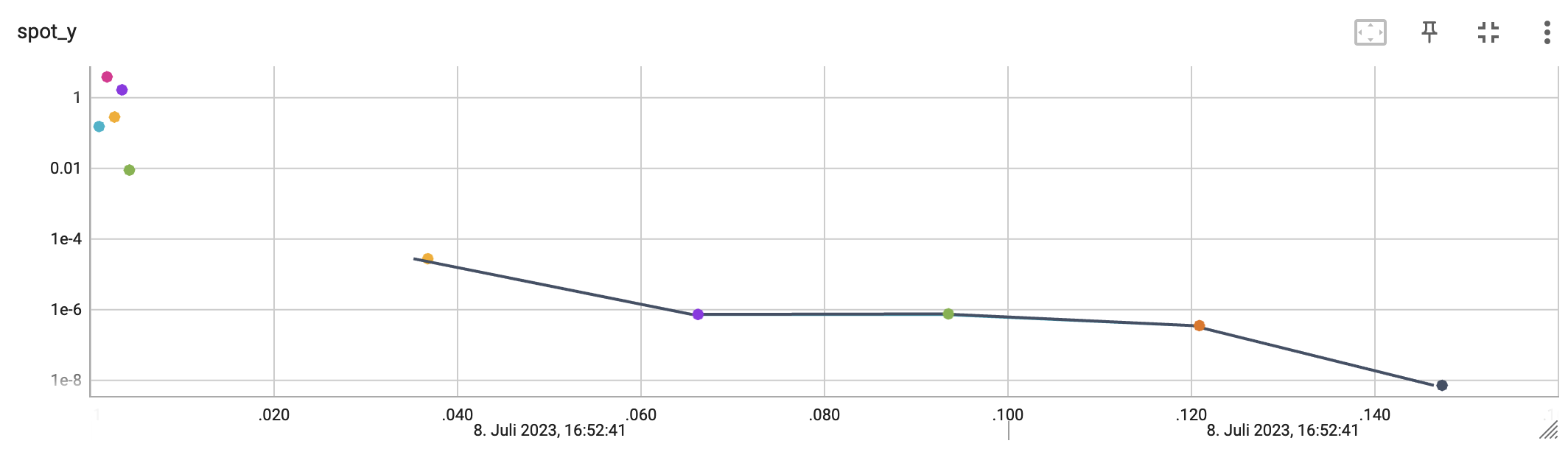

The second TensorBoard visualization shows the input values, i.e., \(x_0\), plotted against the wall time.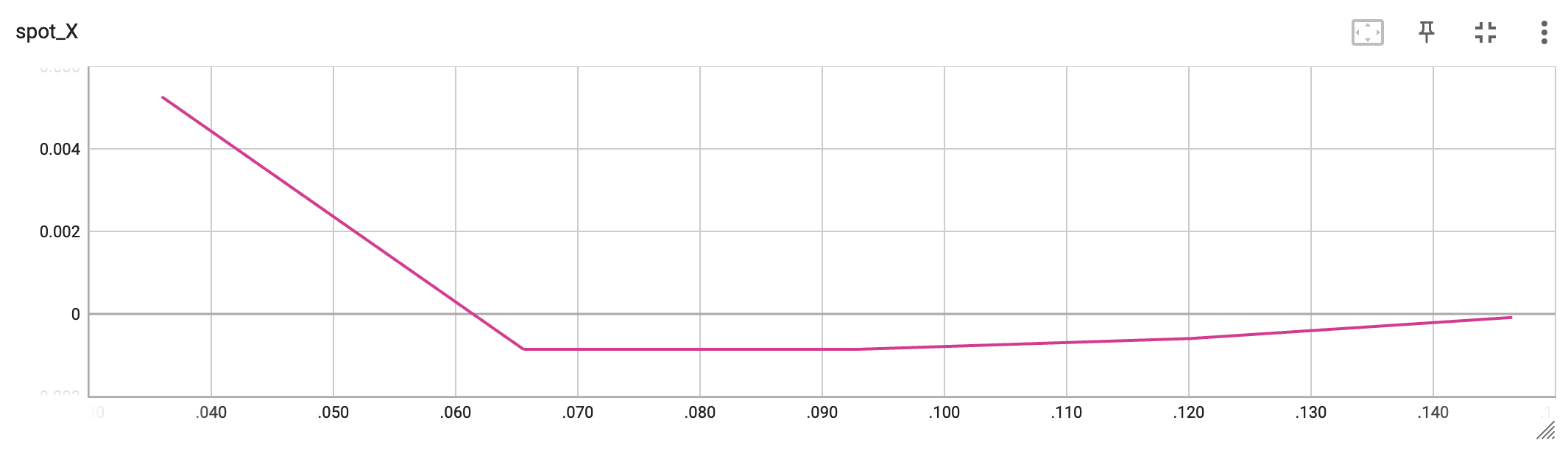

The third TensorBoard plot illustrates how spotpython can be used as a microscope for the internal mechanisms of the surrogate-based optimization process. Here, one important parameter, the learning rate \(\theta\) of the Kriging surrogate is plotted against the number of optimization steps.

TensorBoard visualization of the spotpython process.

7.8 Jupyter Notebook

Note

• The Jupyter-Notebook of this lecture is available on GitHub in the Hyperparameter-Tuning-Cookbook Repository

Bartz-Beielstein, Thomas, and Martina Friese. 2011. “Sequential Parameter Optimization and Optimal Computational Budget Allocation for Noisy Optimization Problems.” Cologne University of Applied Science, Faculty of Computer Science; Engineering Science.

Chen, Chun Hung. 2010. Stochastic simulation optimization: an optimal computing budget allocation. World Scientific.