import numpy as np
import pandas as pd

def randorient(k, p, xi, seed=None):
    # Initialize random number generator with the provided seed
    if seed is not None:
        rng = np.random.default_rng(seed)
    else:
        rng = np.random.default_rng()

    # Step length
    Delta = xi / (p - 1)

    m = k + 1

    # A truncated p-level grid in one dimension
    xs = np.arange(0, 1 - Delta, 1 / (p - 1))
    xsl = len(xs)
    if xsl < 1:
        print(f"xi = {xi}.")
        print(f"p = {p}.")
        print(f"Delta = {Delta}.")
        print(f"p - 1 = {p - 1}.")
        raise ValueError(f"The number of levels xsl is {xsl}, but it must be greater than 0.")

    # Basic sampling matrix
    B = np.vstack((np.zeros((1, k)), np.tril(np.ones((k, k)))))

    # Randomization

    # Matrix with +1s and -1s on the diagonal with equal probability
    Dstar = np.diag(2 * rng.integers(0, 2, size=k) - 1)

    # Random base value
    xstar = xs[rng.integers(0, xsl, size=k)]

    # Permutation matrix
    Pstar = np.zeros((k, k))
    rp = rng.permutation(k)
    for i in range(k):
        Pstar[i, rp[i]] = 1

    # A random orientation of the sampling matrix
    Bstar = (np.ones((m, 1)) @ xstar.reshape(1, -1) + (Delta / 2) * ((2 * B - np.ones((m, k))) @ Dstar + np.ones((m, k)))) @ Pstar

return Bstar1 Introduction: Optimization
1.1 Optimization, Simulation, and Surrogate Modeling
- We will consider the interplay between
- mathematical models,
- numerical approximation,
- simulation,
- computer experiments, and
- field data
- Experimental design will play a key role in our developments, but not in the classical regression and response surface methodology sense
- Challenging real-data/real-simulation examples benefiting from modern surrogate modeling methodology
- We will consider the classical, response surface methodology (RSM) approach, and then move on to more modern approaches
- All approaches are based on surrogates
1.2 Surrogates
- Gathering data is expensive, and sometimes getting exactly the data you want is impossible or unethical
- Surrogate: substitute for the real thing
- In statistics, draws from predictive equations derived from a fitted model can act as a surrogate for the data-generating mechanism
- Benefits of the surrogate approach:
- Surrogate could represent a cheaper way to explore relationships, and entertain “what ifs?”
- Surrogates favor faithful yet pragmatic reproduction of dynamics:
- interpretation,
- establishing causality, or
- identification
- Many numerical simulators are deterministic, whereas field observations are noisy or have measurement error
1.2.1 Costs of Simulation
- Computer simulations are generally cheaper (but not always!) than physical observation
- Some computer simulations can be just as expensive as field experimentation, but computer modeling is regarded as easier because:
- the experimental apparatus is better understood
- more aspects may be controlled.
1.2.2 Mathematical Models and Meta-Models
- Use of mathematical models leveraging numerical solvers has been commonplace for some time
- Mathematical models became more complex, requiring more resources to simulate/solve numerically
- Practitioners increasingly relied on meta-models built off of limited simulation campaigns
1.2.3 Surrogates = Trained Meta-models
- Data collected via expensive computer evaluations tuned flexible functional forms that could be used in lieu of further simulation to
- save money or computational resources;
- cope with an inability to perform future runs (expired licenses, off-line or over-impacted supercomputers)
- Trained meta-models became known as surrogates
1.2.4 Computer Experiments
- Computer experiment: design, running, and fitting meta-models.
- Like an ordinary statistical experiment, except the data are generated by computer codes rather than physical or field observations, or surveys
- Surrogate modeling is statistical modeling of computer experiments
1.2.5 Limits of Mathematical Modeling
- Mathematical biologists, economists and others had reached the limit of equilibrium-based mathematical modeling with cute closed-form solutions
- Stochastic simulations replace deterministic solvers based on FEM, Navier–Stokes or Euler methods
- Agent-based simulation models are used to explore predator-prey (Lotka–Voltera) dynamics, spread of disease, management of inventory or patients in health insurance markets
- Consequence: the distinction between surrogate and statistical model is all but gone
1.2.6 Example: Why Computer Simulations are Necessary
- You can’t seed a real community with Ebola and watch what happens
- If there’s (real) field data, say on a historical epidemic, further experimentation may be almost entirely limited to the mathematical and computer modeling side
- Classical statistical methods offer little guidance
1.2.7 Simulation Requirements
- Simulation should
- enable rich diagnostics to help criticize that models
- understanding its sensitivity to inputs and other configurations
- providing the ability to optimize and
- refine both automatically and with expert intervention
- And it has to do all that while remaining computationally tractable
- One perspective is so-called response surface methods (RSMs):
- a poster child from industrial statistics’ heyday, well before information technology became a dominant industry
1.3 Applications of Surrogate Models
The four most common usages of surrogate models are:
- Augmenting Expensive Simulations: Surrogate models act as a ‘curve fit’ to approximate the results of expensive simulation codes, enabling predictions without rerunning the primary source. This provides significant speed improvements while maintaining useful accuracy.
- Calibration of Predictive Codes: Surrogates bridge the gap between simpler, faster but less accurate models and more accurate, slower models. This multi-fidelity approach allows for improved accuracy without the full computational expense.
- Handling Noisy or Missing Data: Surrogates smooth out random or systematic errors in experimental or computational data, filling gaps and revealing overall trends while filtering out extraneous details.
- Data Mining and Insight Generation: Surrogates help identify functional relationships between variables and their impact on results. They enable engineers to focus on critical variables and visualize data trends effectively.
1.4 The Curse of Dimensionality
The “curse of dimensionality” refers to the exponential increase in computational complexity and data requirements as the number of dimensions (variables) in a problem grows. In high-dimensional spaces, the amount of data needed to maintain the same level of accuracy or coverage increases dramatically. For example, if a one-dimensional space requires \(n\) samples for a certain accuracy, a \(k\)-dimensional space would require \(n^k\) samples. This makes tasks like optimization, sampling, and modeling computationally expensive and often impractical in high-dimensional settings.
1.5 Updating a Surrogate Model
A surrogate model is updated by incorporating new data points, known as infill points, into the model to improve its accuracy and predictive capabilities. This process is iterative and involves the following steps:
- Identify Regions of Interest: The surrogate model is analyzed to determine areas where it is inaccurate or where further exploration is needed. This could be regions with high uncertainty or areas where the model predicts promising results (e.g., potential optima).
- Select Infill Points: Infill points are new data points chosen based on specific criteria, such as:
- Exploitation: Sampling near predicted optima to refine the solution. Exploration: Sampling in regions of high uncertainty to improve the model globally. Balanced Approach: Combining exploitation and exploration to ensure both local and global improvements.
- Evaluate the True Function: The true function (e.g., a simulation or experiment) is evaluated at the selected infill points to obtain their corresponding outputs.
- Update the Surrogate Model: The surrogate model is retrained or updated using the new data, including the infill points, to improve its accuracy.
- Repeat: The process is repeated until the model meets predefined accuracy criteria or the computational budget is exhausted.
Definition 1.1 (Infill Points) Infill points are strategically chosen new data points added to the surrogate model. They are selected to:
- Reduce uncertainty in the model.
- Improve predictions in regions of interest.
- Enhance the model’s ability to identify optima or trends.
The selection of infill points is often guided by infill criteria, such as:
- Expected Improvement (EI): Maximizing the expected improvement over the current best solution.
- Uncertainty Reduction: Sampling where the model’s predictions have high variance.
- Probability of Improvement (PI): Sampling where the probability of improving the current best solution is highest.
The iterative infill-points updating process ensures that the surrogate model becomes increasingly accurate and useful for optimization or decision-making tasks.
1.6 Sampling Plans
1.6.1 Ideas and Concepts
Engineering design often requires the construction of a surrogate model \(\hat{f}\) to approximate the expensive response of a black-box function \(f\). The function \(f(x)\) represents a continuous metric (e.g., quality, cost, or performance) defined over a design space \(D \subset \mathbb{R}^k\), where \(x\) is a \(k\)-dimensional vector of design variables. Since evaluating \(f\) is costly, only a sparse set of samples is used to construct \(\hat{f}\), which can then provide inexpensive predictions for any \(x \in D\).
The process involves:
- Sampling discrete observations:
- Using these samples to construct an approximation \(\hat{f}\).
- Ensuring the surrogate model is well-posed, meaning it is mathematically valid and can generalize predictions effectively.
A sampling plan
\[ X = \left\{ x^{(i)} \in D | i = 1, \ldots, n \right\} \]
determines the spatial arrangement of observations. While some models require a minimum number of data points \(n\), once this threshold is met, a surrogate model can be constructed to approximate \(f\) efficiently.
A well-posed model does not always perform well because its ability to generalize depends heavily on the sampling plan used to collect data. If the sampling plan is poorly designed, the model may fail to capture critical behaviors in the design space. For example:
- Extreme Sampling: Measuring performance only at the extreme values of parameters may miss important behaviors in the center of the design space, leading to incomplete understanding.
- Uneven Sampling: Concentrating samples in certain regions while neglecting others forces the model to extrapolate over unsampled areas, potentially resulting in inaccurate or misleading predictions. Additionally, in some cases, the data may come from external sources or be limited in scope, leaving little control over the sampling plan. This can further restrict the model’s ability to generalize effectively.
1.6.2 The ‘Curse of Dimensionality’ and How to Avoid It
The curse of dimensionality refers to the exponential increase in computational effort as the number of design variables grows. For a one-dimensional space, sampling \(n\) locations may suffice for accurate predictions, but for a \(k\)-dimensional space, the required number of observations increases to \(n^k\). This makes high-dimensional problems computationally expensive and often impractical.
Example 1.1 (Example: Curse of Dimensionality) Consider a simple example where we want to model the cost of a car tire based on its wheel diameter. If we have one variable (wheel diameter), we might need 10 simulations to get a good estimate of the cost. Now, if we add 8 more variables (e.g., tread pattern, rubber type, etc.), the number of simulations required increases to \(10^8\) (10 million). This is because the number of combinations of design variables grows exponentially with the number of dimensions. This means that the computational budget required to evaluate all combinations of design variables becomes infeasible. In this case, it would take 11,416 years to complete the simulations, making it impractical to explore the design space fully.
1.6.3 Physical versus Computational Experiments
Physical experiments are prone to experimental errors from three main sources:
- Human error: Mistakes made by the experimenter.
- Random error: Measurement inaccuracies that vary unpredictably.
- Systematic error: Consistent bias due to flaws in the experimental setup.
The key distinction is repeatability: systematic errors remain constant across repetitions, while random errors vary.
Computational experiments, on the other hand, are deterministic and free from random errors. However, they are still affected by:
- Human error: Bugs in code or incorrect boundary conditions.
- Systematic error: Biases from model simplifications (e.g., inviscid flow approximations) or finite resolution (e.g., insufficient mesh resolution).
The term “noise” is used differently in physical and computational contexts. In physical experiments, it refers to random errors, while in computational experiments, it often refers to systematic errors.
Understanding these differences is crucial for designing experiments and applying techniques like Gaussian process-based approximations. For physical experiments, replication mitigates random errors, but this is unnecessary for deterministic computational experiments.
1.6.4 Designing Preliminary Experiments (Screening)
Minimizing the number of design variables \(x_1, x_2, \dots, x_k\) is crucial before modeling the objective function \(f\). This process, called screening, aims to reduce dimensionality without compromising the analysis. If \(f\) is at least once differentiable over the design domain \(D\), the partial derivative \(\frac{\partial f}{\partial x_i}\) can be used to classify variables:
- Negligible Variables: If \(\frac{\partial f}{\partial x_i} = 0, \, \forall x \in D\), the variable \(x_i\) can be safely neglected.
- Linear Additive Variables: If \(\frac{\partial f}{\partial x_i} = \text{constant} \neq 0, \, \forall x \in D\), the effect of \(x_i\) is linear and additive.
- Nonlinear Variables: If \(\frac{\partial f}{\partial x_i} = g(x_i), \, \forall x \in D\), where \(g(x_i)\) is a non-constant function, \(f\) is nonlinear in \(x_i\).
- Interactive Nonlinear Variables: If \(\frac{\partial f}{\partial x_i} = g(x_i, x_j, \dots), /, \forall x \in D\), where \(g(x_i, x_j, \dots)\) is a function involving interactions with other variables, \(f\) is nonlinear in \(x_i\) and interacts with \(x_j\).
Measuring \(\frac{\partial f}{\partial x_i}\) across the entire design space is often infeasible due to limited budgets. The percentage of time allocated to screening depends on the problem: If many variables are expected to be inactive, thorough screening can significantly improve model accuracy by reducing dimensionality. If most variables are believed to impact the objective, focus should shift to modeling instead. Screening is a trade-off between computational cost and model accuracy, and its effectiveness depends on the specific problem context.
1.6.4.1 Estimating the Distribution of Elementary Effects
In order to simplify the presentation of what follows, we make, without loss of generality, the assumption that the design space \(D = [0, 1]^k\); that is, we normalize all variables into the unit cube. We shall adhere to this convention for the rest of the book and strongly urge the reader to do likewise when implementing any algorithms described here, as this step not only yields clearer mathematics in some cases but also safeguards against scaling issues.
Before proceeding with the description of the Morris algorithm, we need to define an important statistical concept. Let us restrict our design space \(D\) to a \(k\)-dimensional, \(p\)-level full factorial grid, that is,
\[ x_i \in \{0, \frac{1}{p-1}, \frac{2}{p-1}, \dots, 1\}, \quad \text{ for } i = 1, \dots, k. \]
For a given baseline value \(x \in D\), let \(d_i(x)\) denote the elementary effect of \(x_i\), where:
\[ d_i(x) = \frac{f(x_1, \dots, x_i + \Delta, \dots, x_k) - f(x_1, \dots, x_i - \Delta, \dots, x_k)}{2\Delta}, \quad i = 1, \dots, k, \tag{1.1}\] where \(\Delta\) is the step size, which is defined as the distance between two adjacent levels in the grid. In other words, we have:
with \[\Delta = \frac{\xi}{p-1}, \quad \xi \in \mathbb{N}^*, \quad \text{and} \quad x \in D , \text{ such that its components } x_i \leq 1 - \Delta. \]
\(\Delta\) is the step size. The elementary effect \(d_i(x)\) measures the sensitivity of the function \(f\) to changes in the variable \(x_i\) at the point \(x\).
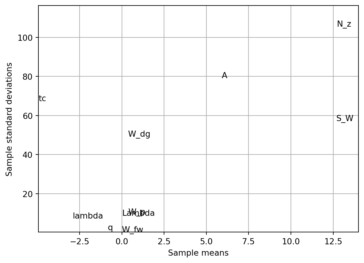
Morris’s method aims to estimate the parameters of the distribution of elementary effects associated with each variable. A large measure of central tendency indicates that a variable has a significant influence on the objective function across the design space, while a large measure of spread suggests that the variable is involved in interactions or contributes to the nonlinearity of \(f\). In practice, the sample mean and standard deviation of a set of \(d_i(x)\) values, calculated in different parts of the design space, are used for this estimation.
To ensure efficiency, the preliminary sampling plan \(X\) should be designed so that each evaluation of the objective function \(f\) contributes to the calculation of two elementary effects, rather than just one (as would occur with a naive random spread of baseline \(x\) values and adding \(\Delta\) to one variable). Additionally, the sampling plan should provide a specified number (e.g., \(r\)) of elementary effects for each variable, independently drawn with replacement. For a detailed discussion on constructing such a sampling plan, readers are encouraged to consult Morris’s original paper (Morris, 1991). Here, we focus on describing the process itself.
The random orientation of the sampling plan \(B\) can be constructed as follows: * Let \(B\) be a \((k+1) \times k\) matrix of 0s and 1s, where for each column \(i\), two rows differ only in their \(i\)-th entries. * Compute a random orientation of \(B\), denoted \(B^*\):
\[ B^* = \left( 1_{k+1,k} x^* + (\Delta/2) \left[ (2B-1_{k+1,k}) D^* + 1_{k+1,k} \right] \right) P^*, \]
where:
- \(D^*\) is a \(k\)-dimensional diagonal matrix with diagonal elements \(\pm 1\) (equal probability),
- \(\mathbf{1}\) is a matrix of 1s,
- \(x^*\) is a randomly chosen point in the \(p\)-level design space (limited by \(\Delta\)),
- \(P^*\) is a \(k \times k\) random permutation matrix with one 1 per column and row.
spotpython provides a Python implementation to compute \(B^*\), see https://github.com/sequential-parameter-optimization/spotPython/blob/main/src/spotpython/utils/effects.py.
Here is the corresponding code:
The code following snippet generates a random orientation of a sampling matrix Bstar using the randorient() function. The input parameters are:
- k = 3: The number of design variables (dimensions).
- p = 3: The number of levels in the grid for each variable.
- xi = 1: A parameter used to calculate the step size Delta.
Step-size calculation is performed as follows: Delta = xi / (p - 1) = 1 / (3 - 1) = 0.5, which determines the spacing between levels in the grid.
Next, random sampling matrix construction is computed:
- A truncated grid is created with levels
[0, 0.5](based on Delta). - A basic sampling matrix B is constructed, which is a lower triangular matrix with 0s and 1s.
Then, randomization is applied:
- Dstar: A diagonal matrix with random entries of +1 or -1.
- xstar: A random starting point from the grid.
- Pstar: A random permutation matrix.
Random orientation is applied to the basic sampling matrix B to create Bstar. This involves scaling, shifting, and permuting the rows and columns of B.
The final output is the matrix Bstar, which represents a random orientation of the sampling plan. Each row corresponds to a sampled point in the design space, and each column corresponds to a design variable.
# Example usage
k = 3
p = 3
xi = 1
Bstar = randorient(k, p, xi)
print(f"Random orientation of the sampling matrix:\n{Bstar}")
Random orientation of the sampling matrix:
[[0.5 0.5 0. ]
[0.5 0. 0. ]
[0. 0. 0. ]
[0. 0. 0.5]]To obtain \(r\) elementary effects for each variable, the screening plan is built from \(r\) random orientations:
\[ X = \begin{pmatrix} B^*_1 \\ B^*_2 \\ \vdots \\ B^*_r \end{pmatrix} \]
The screening plan implementation in Python is as follows (see https://github.com/sequential-parameter-optimization/spotPython/blob/main/src/spotpython/utils/effects.py):
def screeningplan(k, p, xi, r):
    # Empty list to accumulate screening plan rows
    X = []

    for i in range(r):
        X.append(randorient(k, p, xi))

    # Concatenate list of arrays into a single array
    X = np.vstack(X)

    return X
The function screeningplan() generates a screening plan by calling the randorient() function r times. It creates a list of random orientations and then concatenates them into a single array, which represents the screening plan. It works like follows:
The value of the objective function \(f\) is computed for each row of the screening plan matrix \(X\). These values are stored in a column vector \(t\) of size \((r * (k + 1)) \times 1\), where:
r is the number of random orientations.
k is the number of design variables.
The elementary effects are calculated using the following formula:
- For each random orientation, adjacent rows of the screening plan matrix X and their corresponding function values from t are used.
- These values are inserted into Equation 1.1 to compute elementary effects for each variable. An elementary effect measures the sensitivity of the objective function to changes in a specific variable.
Results can be used for a statistical analysis. After collecting a sample of \(r\) elementary effects for each variable:
- The sample mean (central tendency) is computed to indicate the overall influence of the variable.
- The sample standard deviation (spread) is computed to capture variability, which may indicate interactions or nonlinearity.
The results (sample means and standard deviations) are plotted on a chart for comparison. This helps identify which variables have the most significant impact on the objective function and whether their effects are linear or involve interactions.
import numpy as np
from spotpython.utils.effects import screening_plot, screeningplan
from spotpython.fun.objectivefunctions import Analytical
fun = Analytical()
k = 10
p = 10
xi = 1
r = 25
X = screeningplan(k=k, p=p, xi=xi, r=r)  # shape (r x (k+1), k)
value_range = np.array([
    [150, 220,   6, -10, 16, 0.5, 0.08, 2.5, 1700, 0.025],
    [200, 300,  10,  10, 45, 1.0, 0.18, 6.0, 2500, 0.08 ],
])
labels = [
    "S_W", "W_fw", "A", "Lambda",
    "q",   "lambda", "tc", "N_z",
    "W_dg", "W_p"
]
screening_plot(
    X=X,
    fun=fun.fun_wingwt,
    bounds=value_range,
    xi=xi,
    p=p,
    labels=labels,
)
1.7 Designing a Sampling Plan
1.7.1 Stratification
A feature shared by all of the approximation models discussed in Forrester, Sóbester, and Keane (2008) is that they are more accurate in the vicinity of the points where we have evaluated the objective function. In later chapters we will delve into the laws that quantify our decaying trust in the model as we move away from a known, sampled point, but for the purposes of the present discussion we shall merely draw the intuitive conclusion that a uniform level of model accuracy throughout the design space requires a uniform spread of points. A sampling plan possessing this feature is said to be space-filling .
The most straightforward way of sampling a design space in a uniform fashion is by means of a rectangular grid of points. This is the full factorial sampling technique referred to in the section about the curse of dimensionality.
Here is the simplified version of a Python function that will sample the unit hypercube at all levels in all dimensions, with the \(k\)-vector \(q\) containing the number of points required along each dimension, see https://github.com/sequential-parameter-optimization/spotPython/blob/main/src/spotpython/utils/sampling.py.
The variable Edges specifies whether we want the points to be equally spaced from edge to edge (Edges=1) or we want them to be in the centres of \(n = q_1 \times q_2 \times \ldots \times q_k\) bins filling the unit hypercube (for any other value of Edges).
import numpy as np
from typing import Tuple, Optional
import matplotlib.pyplot as plt


def fullfactorial(q, Edges=1) -> np.ndarray:
    """Generates a full factorial sampling plan in the unit cube.

    Args:
        q (list or np.ndarray):
            A list or array containing the number of points along each dimension (k-vector).
        Edges (int, optional):
            Determines spacing of points. If `Edges=1`, points are equally spaced from edge to edge (default).
            Otherwise, points will be in the centers of n = q[0]*q[1]*...*q[k-1] bins filling the unit cube.

    Returns:
        (np.ndarray): Full factorial sampling plan as an array of shape (n, k), where n is the total number of points and k is the number of dimensions.

    Raises:
        ValueError: If any dimension in `q` is less than 2.

    Examples:
        >>> from spotpython.utils.sampling import fullfactorial
        >>> q = [3, 2]
        >>> X = fullfactorial(q, Edges=0)
        >>> print(X)
                [[0.         0.        ]
                [0.         0.75      ]
                [0.41666667 0.        ]
                [0.41666667 0.75      ]
                [0.83333333 0.        ]
                [0.83333333 0.75      ]]
        >>> X = fullfactorial(q, Edges=1)
        >>> print(X)
                [[0.  0. ]
                [0.  1. ]
                [0.5 0. ]
                [0.5 1. ]
                [1.  0. ]
                [1.  1. ]]

    """
    q = np.array(q)
    if np.min(q) < 2:
        raise ValueError("You must have at least two points per dimension.")

    # Total number of points in the sampling plan
    n = np.prod(q)

    # Number of dimensions
    k = len(q)

    # Pre-allocate memory for the sampling plan
    X = np.zeros((n, k))

    # Additional phantom element
    q = np.append(q, 1)

    for j in range(k):
        if Edges == 1:
            one_d_slice = np.linspace(0, 1, q[j])
        else:
            one_d_slice = np.linspace(1 / (2 * q[j]), 1, q[j]) - 1 / (2 * q[j])

        column = np.array([])

        while len(column) < n:
            for ll in range(q[j]):
                column = np.append(column, np.ones(np.prod(q[j + 1 : k])) * one_d_slice[ll])

        X[:, j] = column

    return X
from spotpython.utils.sampling import fullfactorial
q = [3, 2]
X = fullfactorial(q, Edges=0)
print(X)[[0. 0. ]
[0. 0.75 ]
[0.41666667 0. ]
[0.41666667 0.75 ]
[0.83333333 0. ]
[0.83333333 0.75 ]]X = fullfactorial(q, Edges=1)
print(X)[[0. 0. ]
[0. 1. ]
[0.5 0. ]
[0.5 1. ]
[1. 0. ]
[1. 1. ]]The full factorial sampling plan method generates a uniform sampling design by creating a grid of points across all dimensions. For example, calling fullfactorial([3, 4, 5], 1) produces a three-dimensional sampling plan with 3, 4, and 5 levels along each dimension, respectively. While this approach satisfies the uniformity criterion, it has two significant limitations:
Restricted Design Sizes: The method only works for designs where the total number of points \(n\) can be expressed as the product of the number of levels in each dimension, i.e., \(n = q_1 \times q_2 \times \cdots \times q_k\).
Overlapping Projections: When the sampling points are projected onto individual axes, sets of points may overlap, reducing the effectiveness of the sampling plan. This can lead to non-uniform coverage in the projections, which may not fully represent the design space.
1.7.2 Latin Squares and Random Latin Hypercubes
To improve the uniformity of projections for any individual variable, the range of that variable can be divided into a large number of equal-sized bins, and random subsamples of equal size can be generated within these bins. This method is called stratified random sampling. Extending this idea to all dimensions results in a stratified sampling plan, commonly implemented using Latin hypercube sampling.
For two-dimensional discrete variables, a Latin square ensures uniform projections. An \((n \times n)\) Latin square is constructed by filling each row and column with a permutation of \(\{1, 2, \dots, n\}\), ensuring each number appears only once per row and column. For example, for $n = 4 $, a Latin square might look like this:
2   1   3   4
3   2   4   1
1   4   2   3
4   3   1   2
Latin Hypercubes are the multidimensional extension of Latin squares. The design space is divided into equal-sized hypercubes (bins), and one point is placed in each bin. The placement ensures that moving along any axis from an occupied bin does not encounter another occupied bin. This guarantees uniform projections across all dimensions. To construct a Latin hypercube:
Represent the sampling plan as an ( n k ) matrix ( X ), where ( n ) is the number of points and ( k ) is the number of dimensions. Fill each column of ( X ) with random permutations of ( {1, 2, , n} ). Normalize the plan into the unit hypercube ([0, 1]^k). This approach ensures multidimensional stratification and uniformity in projections. Here is the code:
def rlh(n: int, k: int, edges: int = 0) -> np.ndarray:
    # Initialize array
    X = np.zeros((n, k), dtype=float)

    # Fill with random permutations
    for i in range(k):
        X[:, i] = np.random.permutation(n)

    # Adjust normalization based on the edges flag
    if edges == 1:
        # [X=0..n-1] -> [0..1]
        X = X / (n - 1)
    else:
        # Points at true midpoints
        # [X=0..n-1] -> [0.5/n..(n-0.5)/n]
        X = (X + 0.5) / n

    return X
import numpy as np
from spotpython.utils.sampling import rlh
# Generate a 2D Latin hypercube with 5 points and edges=0
X = rlh(n=5, k=2, edges=0)
print(X)[[0.7 0.3]
[0.1 0.1]
[0.5 0.9]
[0.3 0.5]
[0.9 0.7]]import numpy as np
from spotpython.utils.sampling import rlh
# Generate a 2D Latin hypercube with 5 points and edges=1
X = rlh(n=5, k=2, edges=1)
print(X)[[0.75 1. ]
[1. 0.75]
[0. 0.5 ]
[0.25 0.25]
[0.5 0. ]]import numpy as np
import matplotlib.pyplot as plt
from spotpython.utils.sampling import rlh
# Generate a 2D Latin hypercube with 5 points and edges=0
X = rlh(n=5, k=2, edges=0)
# Plot the points
plt.figure(figsize=(6, 6))
plt.scatter(X[:, 0], X[:, 1], color='blue', s=50, label='Hypercube Points')
plt.grid(True, linestyle='--', alpha=0.7)
plt.title('2D Latin Hypercube Sampling (5 Points, Edges=0)')
plt.xlabel('Dimension 1')
plt.ylabel('Dimension 2')
plt.xlim(0, 1)
plt.ylim(0, 1)
plt.legend()
plt.show()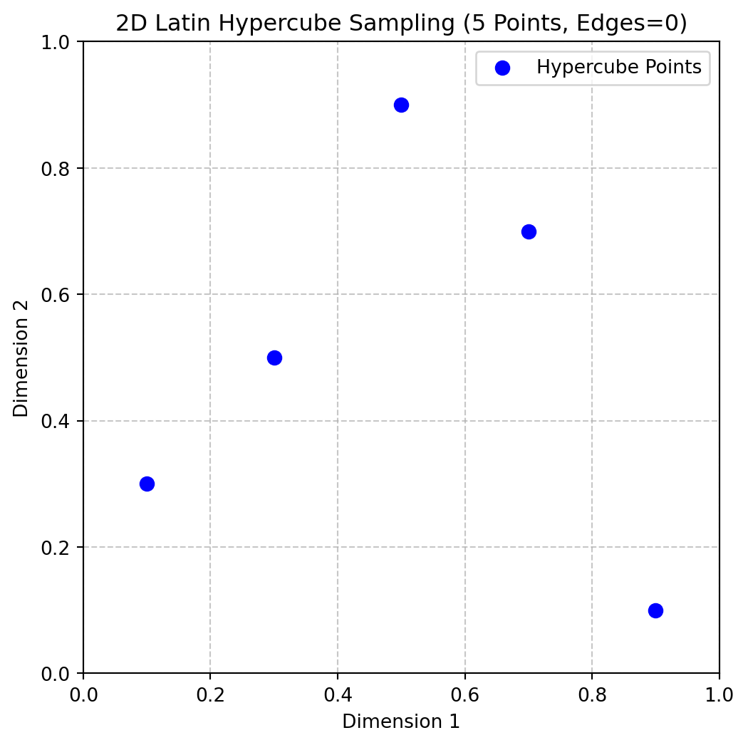
1.7.3 Space-filling Latin Hypercubes
1.7.3.1 Die Funktion jd(X,p)
def jd(X: np.ndarray, p: float = 1.0) -> Tuple[np.ndarray, np.ndarray]:
    """
    Computes and counts the distinct p-norm distances between all pairs of points in X.
    It returns:
    1) A list of distinct distances (sorted), and
    2) A corresponding multiplicity array that indicates how often each distance occurs.

    Args:
        X (np.ndarray):
            A 2D array of shape (n, d) representing n points in d-dimensional space.
        p (float, optional):
            The distance norm to use. p=1 uses the Manhattan (L1) norm, while p=2 uses the
            Euclidean (L2) norm. Defaults to 1.0 (Manhattan norm).

    Returns:
        (np.ndarray, np.ndarray):
            A tuple (J, distinct_d), where:
            - distinct_d is a 1D float array of unique, sorted distances between points.
            - J is a 1D integer array that provides the multiplicity (occurrence count)
              of each distance in distinct_d.
    """
    n = X.shape[0]

    # Allocate enough space for all pairwise distances
    # (n*(n-1))/2 pairs for an n-point set
    pair_count = n * (n - 1) // 2
    d = np.zeros(pair_count, dtype=float)

    # Fill the distance array
    idx = 0
    for i in range(n - 1):
        for j in range(i + 1, n):
            # Compute the p-norm distance
            d[idx] = np.linalg.norm(X[i] - X[j], ord=p)
            idx += 1

    # Find unique distances and their multiplicities
    distinct_d = np.unique(d)
    J = np.zeros_like(distinct_d, dtype=int)
    for i, val in enumerate(distinct_d):
        J[i] = np.sum(d == val)

    return J, distinct_d
1.7.3.2 Die Funktion mm(X1, X2,p)
import numpy as np
from spotpython.utils.sampling import jd
# A small 3-point set in 2D
X = np.array([[0.0, 0.0],[1.0, 1.0],[2.0, 2.0]])
J, distinct_d = jd(X, p=2.0)
print("Distinct distances (d_i):", distinct_d)
print("Occurrences (J_i):", J)
Distinct distances (d_i): [1.41421356 2.82842712]
Occurrences (J_i): [2 1]def mm(X1: np.ndarray, X2: np.ndarray, p: Optional[float] = 1.0) -> int:
"""
Determines which of two sampling plans has better space-filling properties
according to the Morris-Mitchell criterion.
Args:
X1 (np.ndarray): A 2D array representing the first sampling plan.
X2 (np.ndarray): A 2D array representing the second sampling plan.
p (float, optional): The distance metric. p=1 uses Manhattan (L1) distance,
while p=2 uses Euclidean (L2). Defaults to 1.0.
Returns:
int:
- 0 if both plans are identical or equally space-filling
- 1 if X1 is more space-filling
- 2 if X2 is more space-filling
"""
X1_sorted = X1[np.lexsort(np.rot90(X1))]
X2_sorted = X2[np.lexsort(np.rot90(X2))]
if np.array_equal(X1_sorted, X2_sorted):
return 0 # Identical sampling plans
# Compute distance multiplicities for each plan
J1, d1 = jd(X1, p)
J2, d2 = jd(X2, p)
m1, m2 = len(d1), len(d2)
# Construct V1 and V2: alternate distance and negative multiplicity
V1 = np.zeros(2 * m1)
V1[0::2] = d1
V1[1::2] = -J1
V2 = np.zeros(2 * m2)
V2[0::2] = d2
V2[1::2] = -J2
# Trim the longer vector to match the size of the shorter
m = min(m1, m2)
V1 = V1[:m]
V2 = V2[:m]
# Compare element-by-element:
# c[i] = 1 if V1[i] > V2[i], 2 if V1[i] < V2[i], 0 otherwise.
c = (V1 > V2).astype(int) + 2 * (V1 < V2).astype(int)
if np.sum(c) == 0:
# Equally space-filling
return 0
else:
# The first non-zero entry indicates which plan is better
idx = np.argmax(c != 0)
return c[idx]import numpy as np
import matplotlib.pyplot as plt
from spotpython.utils.sampling import mm
# Create two 3-point sampling plans in 2D
X1 = np.array([[0.0, 0.0],[0.5, 0.5],[0.0, 1.0], [1.0, 1.0]])
X2 = np.array([[0.1, 0.1],[0.4, 0.6],[0.1, 0.9], [0.9, 0.9]])
# plot the two plans
plt.scatter(X1[:, 0], X1[:, 1], color='blue', label='Plan 1')
plt.scatter(X2[:, 0], X2[:, 1], color='red', label='Plan 2')
plt.title('Comparison of Two Sampling Plans')
plt.grid()
plt.xlabel('Dimension 1')
plt.ylabel('Dimension 2')
plt.legend()
plt.show()
# Compare which plan has better space-filling (Morris-Mitchell)
better = mm(X1, X2, p=2.0)
print(better)
# Prints either 0, 1, or 2 depending on which plan is more space-filling.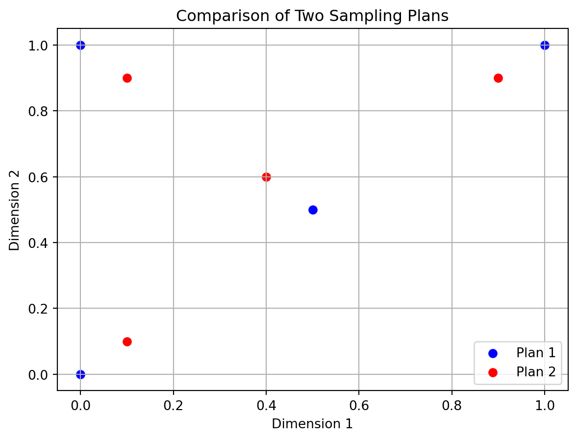
11.7.3.3 Die Funktion mmphi(X,q,p)
def mmphi(X: np.ndarray, q: Optional[float] = 2.0, p: Optional[float] = 1.0) -> float:
    """
    Calculates the Morris-Mitchell sampling plan quality criterion.

    Args:
        X (np.ndarray):
            A 2D array representing the sampling plan, where each row is a point in
            d-dimensional space (shape: (n, d)).
        q (float, optional):
            Exponent used in the computation of the metric. Defaults to 2.0.
        p (float, optional):
            The distance norm to use. For example, p=1 is Manhattan (L1),
            p=2 is Euclidean (L2). Defaults to 1.0.

    Returns:
        float:
            The space-fillingness metric Phiq. Larger values typically indicate a more
            space-filling plan according to the Morris-Mitchell criterion.
    """
    # Compute the distance multiplicities: J, and unique distances: d
    J, d = jd(X, p)

    # Summation of J[i] * d[i]^(-q), then raised to 1/q
    # This follows the Morris-Mitchell definition.
    Phiq = np.sum(J * (d ** (-q))) ** (1.0 / q)
    return Phiq
import numpy as np
from spotpython.utils.sampling import mmphi
# Two simple sampling plans from above
quality1 = mmphi(X1, q=2, p=2)
quality2 = mmphi(X2, q=2, p=2)
print(f"Quality of sampling plan X1: {quality1}")
print(f"Quality of sampling plan X2: {quality2}")Quality of sampling plan X1: 2.91547594742265
Quality of sampling plan X2: 3.9171620462692151.7.3.3.1 Die Funktion mmsort(X3D,p)
def mmsort(X3D: np.ndarray, p: Optional[float] = 1.0) -> np.ndarray:
    """
    Ranks multiple sampling plans stored in a 3D array according to the
    Morris-Mitchell criterion, using a simple bubble sort.

    Args:
        X3D (np.ndarray):
            A 3D NumPy array of shape (n, d, m), where m is the number of
            sampling plans, and each plan is an (n, d) matrix of points.
        p (float, optional):
            The distance metric to use. p=1 for Manhattan (L1), p=2 for
            Euclidean (L2). Defaults to 1.0.

    Returns:
        np.ndarray:
            A 1D integer array of length m that holds the plan indices in
            ascending order of space-filling quality. The first index in the
            returned array corresponds to the most space-filling plan.

    Notes:
        Many thanks to the original author of this code, A Sobester, for providing the original Matlab code under the GNU Licence. Original Matlab Code: Copyright 2007 A Sobester:
        "This program is free software: you can redistribute it and/or modify  it
        under the terms of the GNU Lesser General Public License as published by
        the Free Software Foundation, either version 3 of the License, or any
        later version.
        This program is distributed in the hope that it will be useful, but
        WITHOUT ANY WARRANTY; without even the implied warranty of
        MERCHANTABILITY or FITNESS FOR A PARTICULAR PURPOSE.  See the GNU Lesser
        General Public License for more details.
        You should have received a copy of the GNU General Public License and GNU
        Lesser General Public License along with this program. If not, see
        <http://www.gnu.org/licenses/>."
    """
    # Number of plans (m)
    m = X3D.shape[2]

    # Create index array (1-based to match original MATLAB convention)
    Index = np.arange(1, m + 1)

    swap_flag = True
    while swap_flag:
        swap_flag = False
        i = 0
        while i < m - 1:
            # Compare plan at Index[i] vs. Index[i+1] using mm()
            # Note: subtract 1 from each index to convert to 0-based array indexing
            if mm(X3D[:, :, Index[i] - 1], X3D[:, :, Index[i + 1] - 1], p) == 2:
                # Swap indices if the second plan is more space-filling
                Index[i], Index[i + 1] = Index[i + 1], Index[i]
                swap_flag = True
            i += 1

    return Index
import numpy as np
from spotpython.utils.sampling import mmsort
# Suppose we have two 3-point sampling plans X1 and X1 from above
X3D = np.stack([X1, X2], axis=2)
# Sort them using the Morris-Mitchell criterion with p=2
ranking = mmsort(X3D, p=2.0)
print(ranking)
# It prints [1, 2] indicating that X1 is more space-filling than X2.[1 2]1.7.3.4 Die Funktion perturb(X,PertNum=1)
def perturb(X: np.ndarray, PertNum: Optional[int] = 1) -> np.ndarray:
    """
    Performs a specified number of random element swaps on a sampling plan.
    If the plan is a Latin hypercube, the result remains a valid Latin hypercube.

    Args:
        X (np.ndarray):
            A 2D array (sampling plan) of shape (n, k), where each row is a point
            and each column is a dimension.
        PertNum (int, optional):
            The number of element swaps (perturbations) to perform. Defaults to 1.

    Returns:
        np.ndarray:
            The perturbed sampling plan, identical in shape to the input, with
            one or more random column swaps executed.
    """
    # Get dimensions of the plan
    n, k = X.shape
    if n < 2 or k < 2:
        raise ValueError("Latin hypercubes require at least 2 points and 2 dimensions")

    for _ in range(PertNum):
        # Pick a random column
        col = int(np.floor(np.random.rand() * k))

        # Pick two distinct row indices
        el1, el2 = 0, 0
        while el1 == el2:
            el1 = int(np.floor(np.random.rand() * n))
            el2 = int(np.floor(np.random.rand() * n))

        # Swap the two selected elements in the chosen column
        X[el1, col], X[el2, col] = X[el2, col], X[el1, col]

    return X
import numpy as np
from spotpython.utils.sampling import perturb
# Create a simple 4x2 sampling plan
X_original = np.array([[1, 3],[2, 4],[3, 1],[4, 2]])
print("Original Sampling Plan:")
print(X_original)
print("Perturbed Sampling Plan:")
X_perturbed = perturb(X_original, PertNum=1)
print(X_perturbed)Original Sampling Plan:
[[1 3]
[2 4]
[3 1]
[4 2]]
Perturbed Sampling Plan:
[[1 1]
[2 4]
[3 3]
[4 2]]1.7.3.5 The function mmlhs(X_start, population, iterations, q=2.0, plot=False)
def mmlhs(X_start: np.ndarray, population: int, iterations: int, q: Optional[float] = 2.0, plot=False) -> np.ndarray:
    """
    Performs an evolutionary search (using perturbations) to find a Morris-Mitchell
    optimal Latin hypercube, starting from an initial plan X_start.

    This function does the following:
      1. Initializes a "best" Latin hypercube (X_best) from the provided X_start.
      2. Iteratively perturbs X_best to create offspring.
      3. Evaluates the space-fillingness of each offspring via the Morris-Mitchell
         metric (using mmphi).
      4. Updates the best plan whenever a better offspring is found.

    Args:
        X_start (np.ndarray):
            A 2D array of shape (n, k) providing the initial Latin hypercube
            (n points in k dimensions).
        population (int):
            Number of offspring to create in each generation.
        iterations (int):
            Total number of generations to run the evolutionary search.
        q (float, optional):
            The exponent used by the Morris-Mitchell space-filling criterion.
            Defaults to 2.0.
        plot (bool, optional):
            If True, a simple scatter plot of the first two dimensions will be
            displayed at each iteration. Only if k >= 2. Defaults to False.

    Returns:
        np.ndarray:
            A 2D array representing the most space-filling Latin hypercube found
            after all iterations, of the same shape as X_start.
    """
    n = X_start.shape[0]
    if n < 2:
        raise ValueError("Latin hypercubes require at least 2 points")
    k = X_start.shape[1]
    if k < 2:
        raise ValueError("Latin hypercubes are not defined for dim k < 2")

    # Initialize best plan and its metric
    X_best = X_start.copy()
    Phi_best = mmphi(X_best, q=q)

    # After 85% of iterations, reduce the mutation rate to 1
    leveloff = int(np.floor(0.85 * iterations))

    for it in range(1, iterations + 1):
        # Decrease number of mutations over time
        if it < leveloff:
            mutations = int(round(1 + (0.5 * n - 1) * (leveloff - it) / (leveloff - 1)))
        else:
            mutations = 1

        X_improved = X_best.copy()
        Phi_improved = Phi_best

        # Create offspring, evaluate, and keep the best
        for _ in range(population):
            X_try = perturb(X_best.copy(), mutations)
            Phi_try = mmphi(X_try, q=q)

            if Phi_try < Phi_improved:
                X_improved = X_try
                Phi_improved = Phi_try

        # Update the global best if we found a better plan
        if Phi_improved < Phi_best:
            X_best = X_improved
            Phi_best = Phi_improved

        # Simple visualization of the first two dimensions
        if plot and (X_best.shape[1] >= 2):
            plt.clf()
            plt.scatter(X_best[:, 0], X_best[:, 1], marker="o")
            plt.grid(True)
            plt.title(f"Iteration {it} - Current Best Plan")
            plt.pause(0.01)

    return X_best
import numpy as np
from spotpython.utils.sampling import mmlhs
# Suppose we have an initial 4x2 plan
X_start = np.array([[0.1, 0.3],[.1, .4],[.2, .9],[.9, .2]])
print("Initial plan:")
print(X_start)
# Search for a more space-filling plan
X_opt = mmlhs(X_start, population=10, iterations=100, q=2)
print("Optimized plan:")
print(X_opt)
# Plot the initial and optimized plans
import matplotlib.pyplot as plt
plt.scatter(X_start[:, 0], X_start[:, 1], color='blue', label='Initial Plan')
plt.scatter(X_opt[:, 0], X_opt[:, 1], color='red', label='Optimized Plan')
plt.title('Comparison of Initial and Optimized Plans')
plt.xlabel('Dimension 1')
plt.ylabel('Dimension 2')
plt.grid()
# plot legend outside the plot
plt.legend(loc='upper left', bbox_to_anchor=(1, 1))
plt.xlim(0, 1)
plt.ylim(0, 1)
plt.show()Initial plan:
[[0.1 0.3]
[0.1 0.4]
[0.2 0.9]
[0.9 0.2]]
Optimized plan:
[[0.9 0.3]
[0.1 0.9]
[0.2 0.4]
[0.1 0.2]]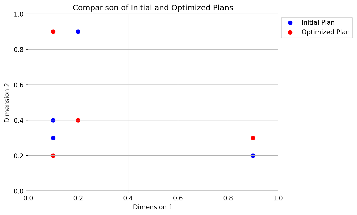
1.7.3.6 Die Funktion bestlh()
def bestlh(n: int, k: int, population: int, iterations: int, p=1, plot=False, verbosity=0, edges=0, q_list=[1, 2, 5, 10, 20, 50, 100]) -> np.ndarray:
    """
    Generates an optimized Latin hypercube by evolving the Morris-Mitchell
    criterion across multiple exponents (q values) and selecting the best plan.

    Args:
        n (int):
            Number of points required in the Latin hypercube.
        k (int):
            Number of design variables (dimensions).
        population (int):
            Number of offspring in each generation of the evolutionary search.
        iterations (int):
            Number of generations for the evolutionary search.
        p (int, optional):
            The distance norm to use. p=1 for Manhattan (L1), p=2 for Euclidean (L2).
            Defaults to 1 (faster than 2).
        plot (bool, optional):
            If True, a scatter plot of the optimized plan in the first two dimensions
            will be displayed. Only if k>=2.  Defaults to False.
        verbosity (int, optional):
            Verbosity level. 0 is silent, 1 prints the best q value found. Defaults to 0.
        edges (int, optional):
            If 1, places centers of the extreme bins at the domain edges ([0,1]).
            Otherwise, bins are fully contained within the domain, i.e. midpoints.
            Defaults to 0.
        q_list (list, optional):
            A list of q values to optimize. Defaults to [1, 2, 5, 10, 20, 50, 100].
            These values are used to evaluate the space-fillingness of the Latin
            hypercube. The best plan is selected based on the lowest mmphi value.

    Returns:
        np.ndarray:
            A 2D array of shape (n, k) representing an optimized Latin hypercube.

    Notes:
        Many thanks to the original author of this code, A Sobester, for providing the original Matlab code under the GNU Licence. Original Matlab Code: Copyright 2007 A Sobester:
        "This program is free software: you can redistribute it and/or modify  it
        under the terms of the GNU Lesser General Public License as published by
        the Free Software Foundation, either version 3 of the License, or any
        later version.
        This program is distributed in the hope that it will be useful, but
        WITHOUT ANY WARRANTY; without even the implied warranty of
        MERCHANTABILITY or FITNESS FOR A PARTICULAR PURPOSE.  See the GNU Lesser
        General Public License for more details.
        You should have received a copy of the GNU General Public License and GNU
        Lesser General Public License along with this program. If not, see
        <http://www.gnu.org/licenses/>."
    """
    if n < 2:
        raise ValueError("Latin hypercubes require at least 2 points")
    if k < 2:
        raise ValueError("Latin hypercubes are not defined for dim k < 2")

    # A list of exponents (q) to optimize

    # Start with a random Latin hypercube
    X_start = rlh(n, k, edges=edges)

    # Allocate a 3D array to store the results for each q
    # (shape: (n, k, number_of_q_values))
    X3D = np.zeros((n, k, len(q_list)))

    # Evolve the plan for each q in q_list
    for i, q_val in enumerate(q_list):
        if verbosity > 0:
            print(f"Now optimizing for q={q_val}...")
        X3D[:, :, i] = mmlhs(X_start, population, iterations, q_val)

    # Sort the set of evolved plans according to the Morris-Mitchell criterion
    index_order = mmsort(X3D, p=p)

    # index_order is a 1-based array of plan indices; the first element is the best
    best_idx = index_order[0] - 1
    if verbosity > 0:
        print(f"Best lh found using q={q_list[best_idx]}...")

    # The best plan in 3D array order
    X = X3D[:, :, best_idx]

    # Plot the first two dimensions
    if plot and (k >= 2):
        plt.scatter(X[:, 0], X[:, 1], c="r", marker="o")
        plt.title(f"Morris-Mitchell optimum plan found using q={q_list[best_idx]}")
        plt.xlabel("x_1")
        plt.ylabel("x_2")
        plt.grid(True)
        plt.show()

    return X
import numpy as np
from spotpython.utils.sampling import bestlh
Xbestlh= bestlh(n=5, k=2, population=5, iterations=10)
# plot the bestlh
import matplotlib.pyplot as plt
plt.scatter(Xbestlh[:, 0], Xbestlh[:, 1], color='red', label='Best Latin Hypercube')
plt.title('Best Latin Hypercube Sampling')
plt.grid()
plt.xlabel('Dimension 1')
plt.ylabel('Dimension 2')
# plot legend outside the plot
plt.legend(loc='upper left', bbox_to_anchor=(1, 1))
plt.xlim(0, 1)
plt.ylim(0, 1)
plt.show()
1.7.3.7 Die Funktion phisort(X3D,q,p)
def phisort(X3D: np.ndarray, q: Optional[float] = 2.0, p: Optional[float] = 1.0) -> np.ndarray:
    """
    Ranks multiple sampling plans stored in a 3D array by the Morris-Mitchell
    numerical quality metric (mmphi). Uses a simple bubble-sort:
    sampling plans with smaller mmphi values are placed first in the index array.

    Args:
        X3D (np.ndarray):
            A 3D array of shape (n, d, m), where m is the number of sampling plans.
        q (float, optional):
            Exponent for the mmphi metric. Defaults to 2.0.
        p (float, optional):
            Distance norm for mmphi. p=1 is Manhattan; p=2 is Euclidean. Defaults to 1.0.

    Returns:
        np.ndarray:
            A 1D integer array of length m, giving the plan indices in ascending
            order of mmphi. The first index in the returned array corresponds
            to the numerically lowest mmphi value.
    """
    # Number of 2D sampling plans
    m = X3D.shape[2]

    # Create a 1-based index array
    Index = np.arange(1, m + 1)

    # Bubble-sort: plan with lower mmphi() climbs toward the front
    swap_flag = True
    while swap_flag:
        swap_flag = False
        for i in range(m - 1):
            # Retrieve mmphi values for consecutive plans
            val_i = mmphi(X3D[:, :, Index[i] - 1], q=q, p=p)
            val_j = mmphi(X3D[:, :, Index[i + 1] - 1], q=q, p=p)

            # Swap if the left plan's mmphi is larger (i.e. 'worse')
            if val_i > val_j:
                Index[i], Index[i + 1] = Index[i + 1], Index[i]
                swap_flag = True

    return Index
import numpy as np
from spotpython.utils.sampling import phisort
X1 = bestlh(n=5, k=2, population=5, iterations=10)
X2 = bestlh(n=5, k=2, population=15, iterations=20)
X3 = bestlh(n=5, k=2, population=25, iterations=30)
# Map X1 and X2 so that X3D has the two sampling plans in X3D[:, :, 0] and X3D[:, :, 1]
X3D = np.array([X1, X2])
print(phisort(X3D))
X3D = np.array([X3, X2])
print(phisort(X3D))[1 2]
[2 1]
Goals
- How to choose models and optimizers for solving real-world problems
- How to use simulation to understand and improve processes
1.8 Jupyter Notebook
Note
- The Jupyter-Notebook of this lecture is available on GitHub in the Hyperparameter-Tuning-Cookbook Repository