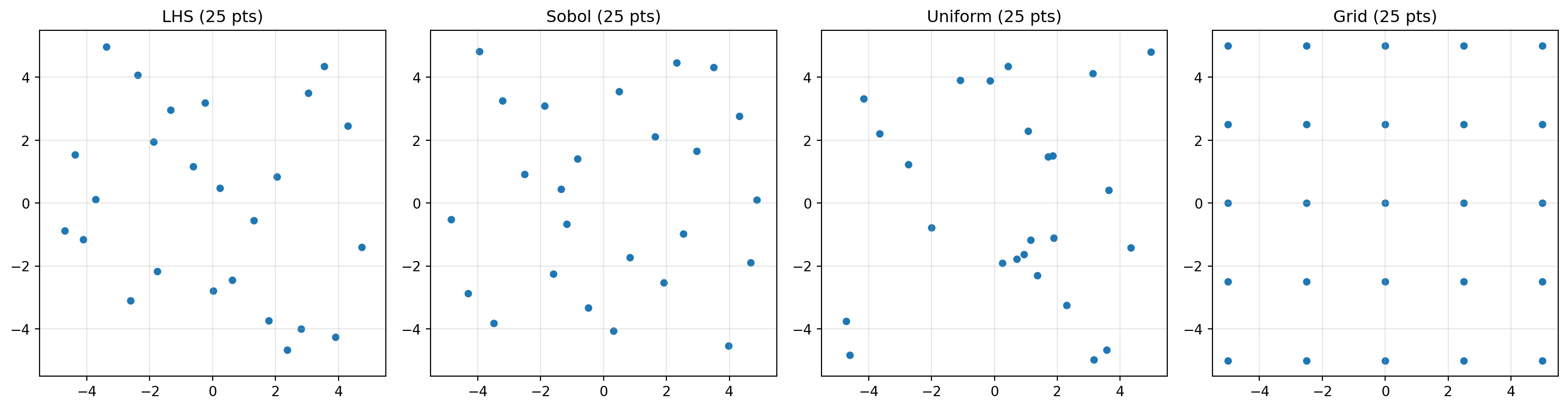
Sampling and Experimental Designs

Space-filling designs for the initial evaluation phase: LHS, Sobol, grid, and more.

Before fitting a surrogate, spotoptim evaluates the objective at an initial set of design points. These points should be spread evenly across the search space to give the surrogate a good starting picture of the response surface.

The spotoptim.sampling.design module provides several design generators. All accept bounds, n_design (number of points), and an optional seed.

Latin Hypercube Sampling (Default)

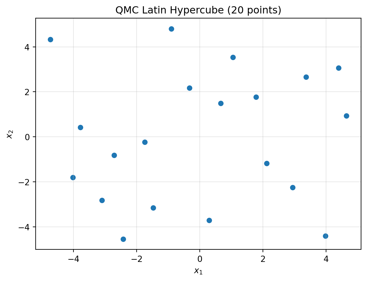
Latin Hypercube Sampling (LHS) ensures each variable’s marginal distribution is well-covered. spotoptim uses the QMC variant by default.

import numpy as np
import matplotlib.pyplot as plt
from spotoptim.sampling.design import generate_qmc_lhs_design

bounds = [(-5, 5), (-5, 5)]
X = generate_qmc_lhs_design(bounds, n_design=20, seed=0)

plt.scatter(X[:, 0], X[:, 1], s=30)
plt.xlabel("$x_1$")
plt.ylabel("$x_2$")
plt.title("QMC Latin Hypercube (20 points)")
plt.grid(True, alpha=0.3)
plt.show()

print(f"Shape: {X.shape}")

Shape: (20, 2)

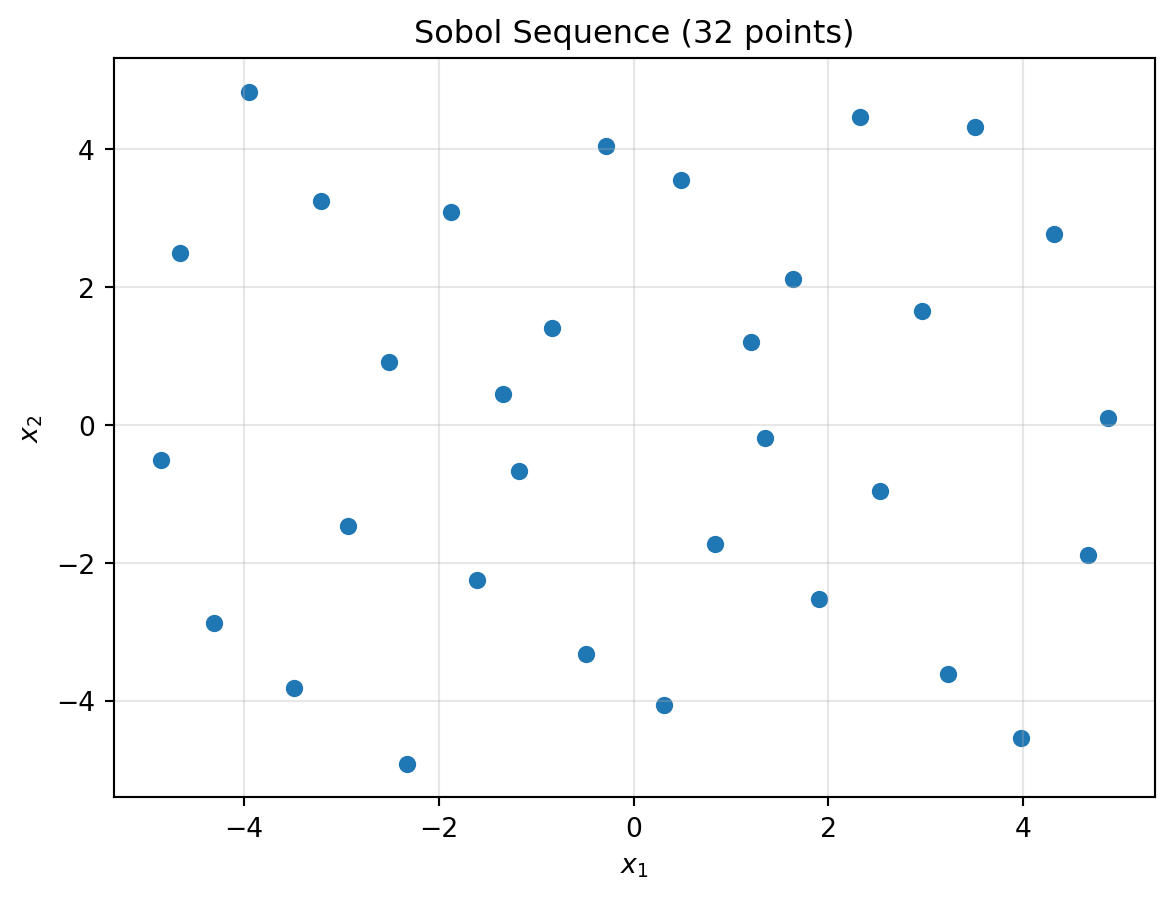
Sobol Sequences

Sobol sequences are quasi-random low-discrepancy sequences. They provide very uniform coverage, especially useful in higher dimensions.

import numpy as np
import matplotlib.pyplot as plt
from spotoptim.sampling.design import generate_sobol_design

bounds = [(-5, 5), (-5, 5)]
X = generate_sobol_design(bounds, n_design=32, seed=0)

plt.scatter(X[:, 0], X[:, 1], s=30)
plt.xlabel("$x_1$")
plt.ylabel("$x_2$")
plt.title("Sobol Sequence (32 points)")
plt.grid(True, alpha=0.3)
plt.show()

print(f"Shape: {X.shape}")

Shape: (32, 2)

Grid Design

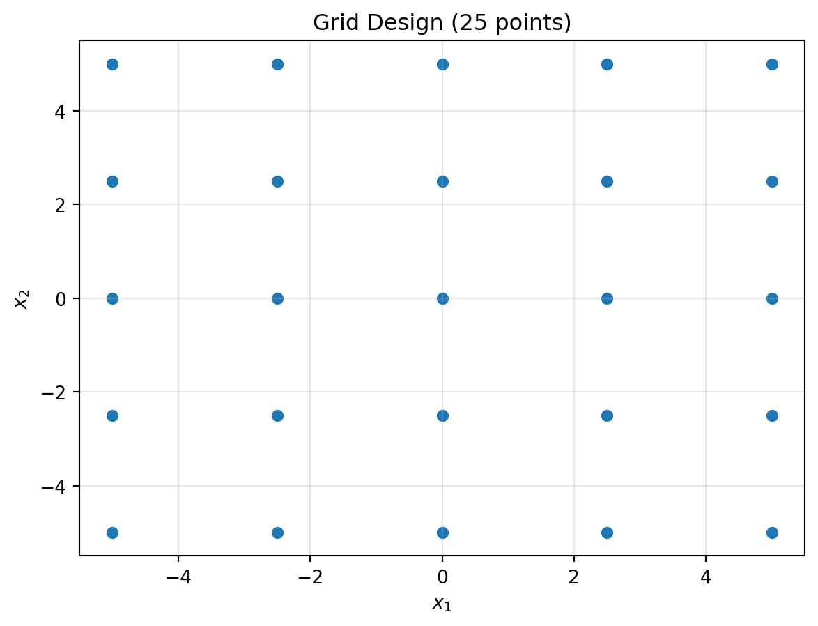
A regular grid with equal spacing per dimension. The actual number of points is \(\lfloor n^{1/d} \rfloor^d\) where \(n\) is the requested count and \(d\) is the number of dimensions.

import numpy as np
import matplotlib.pyplot as plt
from spotoptim.sampling.design import generate_grid_design

bounds = [(-5, 5), (-5, 5)]
X = generate_grid_design(bounds, n_design=25, seed=0)

plt.scatter(X[:, 0], X[:, 1], s=30)
plt.xlabel("$x_1$")
plt.ylabel("$x_2$")
plt.title(f"Grid Design ({X.shape[0]} points)")
plt.grid(True, alpha=0.3)
plt.show()

print(f"Shape: {X.shape}")

Shape: (25, 2)

Uniform Random

Simple uniform random sampling within the bounds. Less structured than LHS or Sobol, but sometimes useful as a baseline.

import numpy as np
import matplotlib.pyplot as plt
from spotoptim.sampling.design import generate_uniform_design

bounds = [(-5, 5), (-5, 5)]
X = generate_uniform_design(bounds, n_design=20, seed=0)

plt.scatter(X[:, 0], X[:, 1], s=30)
plt.xlabel("$x_1$")
plt.ylabel("$x_2$")
plt.title("Uniform Random (20 points)")
plt.grid(True, alpha=0.3)
plt.show()

print(f"Shape: {X.shape}")

Shape: (20, 2)

Clustered Design

Generates points clustered around a specified number of cluster centers. Useful for testing how optimizers handle non-uniform initial distributions.

import numpy as np
import matplotlib.pyplot as plt
from spotoptim.sampling.design import generate_clustered_design

bounds = [(-5, 5), (-5, 5)]
X = generate_clustered_design(bounds, n_design=30, n_clusters=3, seed=0)

plt.scatter(X[:, 0], X[:, 1], s=30)
plt.xlabel("$x_1$")
plt.ylabel("$x_2$")
plt.title("Clustered Design (30 points, 3 clusters)")
plt.grid(True, alpha=0.3)
plt.show()

print(f"Shape: {X.shape}")

Shape: (30, 2)

Comparing Designs Side by Side

import numpy as np
import matplotlib.pyplot as plt
from spotoptim.sampling.design import (
    generate_qmc_lhs_design,
    generate_sobol_design,
    generate_uniform_design,
    generate_grid_design,
)

bounds = [(-5, 5), (-5, 5)]
designs = {
    "LHS": generate_qmc_lhs_design(bounds, 25, seed=0),
    "Sobol": generate_sobol_design(bounds, 25, seed=0),
    "Uniform": generate_uniform_design(bounds, 25, seed=0),
    "Grid": generate_grid_design(bounds, 25, seed=0),
}

fig, axes = plt.subplots(1, 4, figsize=(16, 4))
for ax, (name, X) in zip(axes, designs.items()):
    ax.scatter(X[:, 0], X[:, 1], s=20)
    ax.set_title(f"{name} ({X.shape[0]} pts)")
    ax.set_xlim(-5.5, 5.5)
    ax.set_ylim(-5.5, 5.5)
    ax.set_aspect("equal")
    ax.grid(True, alpha=0.3)
plt.tight_layout()
plt.show()

Using a Custom Initial Design

You can pass a pre-computed initial design to SpotOptim.optimize() via the X0 parameter:

import numpy as np
from spotoptim import SpotOptim
from spotoptim.function import sphere
from spotoptim.sampling.design import generate_sobol_design

bounds = [(-5, 5), (-5, 5)]
X0 = generate_sobol_design(bounds, n_design=16, seed=0)

opt = SpotOptim(
    fun=sphere,
    bounds=bounds,
    max_iter=25,
    n_initial=16,
    seed=0,
)
result = opt.optimize(X0=X0)

print(f"Best f(x) : {result.fun:.6f}")
print(f"Evaluations: {result.nfev}")

Best f(x) : 0.000001
Evaluations: 25