Multi-Objective Optimization

Pareto fronts, desirability functions, and multi-objective test problems.

spotoptim supports multi-objective optimization through Pareto efficiency analysis, a library of standard test functions, and a scalarization mechanism that lets the surrogate-based optimizer handle vector-valued objectives.

---

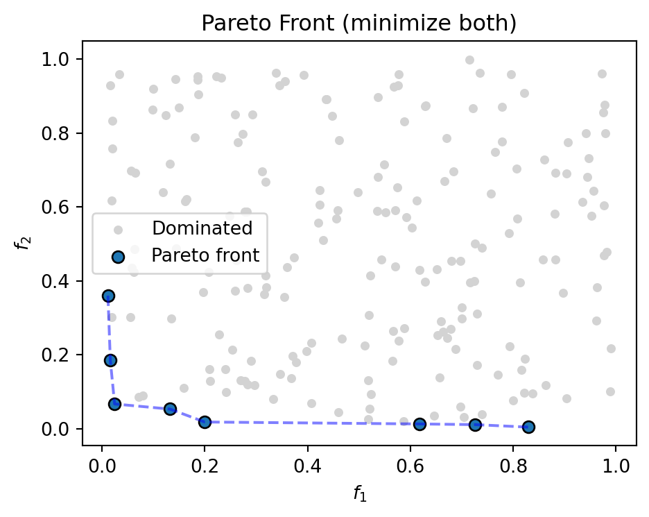
Pareto Efficiency

A solution is Pareto-efficient when no other solution improves one objective without worsening another. The is_pareto_efficient function accepts an \((N, M)\) cost array and returns a boolean mask identifying the non-dominated points.

import numpy as np
from spotoptim.mo.pareto import is_pareto_efficient

np.random.seed(0)
costs = np.random.rand(80, 2)          # 80 random points, 2 objectives
mask = is_pareto_efficient(costs, minimize=True)

print(f"Total points   : {len(costs)}")
print(f"Pareto-efficient: {mask.sum()}")
print(f"Dominated      : {(~mask).sum()}")

Total points   : 80
Pareto-efficient: 6
Dominated      : 74

The function works for any number of objectives. Pass minimize=False when higher values are preferred.

Plotting the Pareto front

import numpy as np
import matplotlib.pyplot as plt
from spotoptim.mo.pareto import is_pareto_efficient

np.random.seed(0)
costs = np.random.rand(200, 2)
mask = is_pareto_efficient(costs, minimize=True)

front = costs[mask]
order = np.argsort(front[:, 0])
front = front[order]

plt.figure(figsize=(5, 4))
plt.scatter(costs[~mask, 0], costs[~mask, 1],
            c="lightgray", s=15, label="Dominated")
plt.scatter(front[:, 0], front[:, 1],
            c="tab:blue", s=40, edgecolor="k", label="Pareto front")
plt.plot(front[:, 0], front[:, 1], "b--", alpha=0.5)
plt.xlabel("$f_1$")
plt.ylabel("$f_2$")
plt.title("Pareto Front (minimize both)")
plt.legend()
plt.tight_layout()
plt.show()
print(f"Pareto front size: {mask.sum()}")

Pareto front size: 8

---

Multi-Objective Test Functions

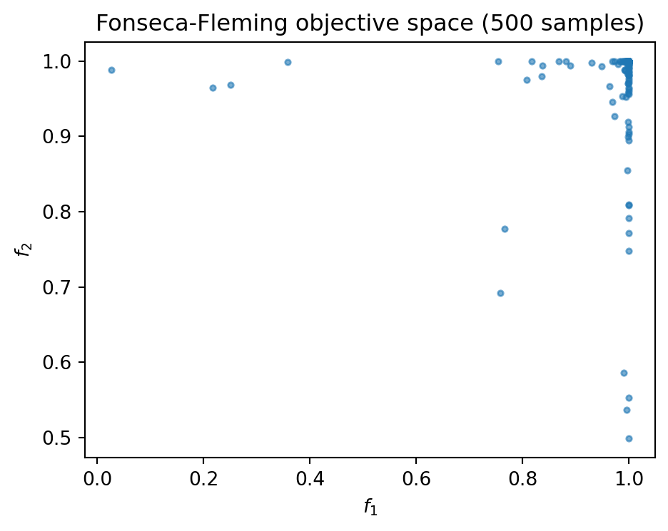
spotoptim ships with several classical bi-objective test functions in spotoptim.function. Each accepts an input array of shape \((n_\text{samples},\; n_\text{features})\) and returns objectives of shape \((n_\text{samples},\; 2)\).

Function	Domain	Pareto front	Min features
zdt1	\([0,1]^n\)	Convex	2
zdt2	\([0,1]^n\)	Non-convex	2
zdt3	\([0,1]^n\)	Disconnected	2
fonseca_fleming	\([-4,4]^n\)	Concave	1
schaffer_n1	\([-10,10]\)	Convex	1
kursawe	\([-5,5]^n\)	Disconnected	2

See Built-in Test Functions for single-objective functions and the full catalogue.

ZDT1

import numpy as np
from spotoptim.function import zdt1

np.random.seed(0)
X = np.random.rand(50, 30)             # 50 samples, 30 variables
Y = zdt1(X)

print(f"Input shape : {X.shape}")
print(f"Output shape: {Y.shape}")
print(f"f1 range    : [{Y[:, 0].min():.3f}, {Y[:, 0].max():.3f}]")
print(f"f2 range    : [{Y[:, 1].min():.3f}, {Y[:, 1].max():.3f}]")

Input shape : (50, 30)
Output shape: (50, 2)
f1 range    : [0.003, 0.990]
f2 range    : [2.256, 6.221]

Fonseca-Fleming

The Fonseca-Fleming function has a concave Pareto front. Both objectives lie in \([0, 1]\):

\[ f_1(\mathbf{x}) = 1 - \exp\!\Bigl(-\sum_{i=1}^{n}(x_i - 1/\sqrt{n})^2\Bigr),\qquad f_2(\mathbf{x}) = 1 - \exp\!\Bigl(-\sum_{i=1}^{n}(x_i + 1/\sqrt{n})^2\Bigr) \]

import numpy as np
import matplotlib.pyplot as plt
from spotoptim.function import fonseca_fleming

np.random.seed(0)
X = np.random.uniform(-4, 4, size=(500, 3))
Y = fonseca_fleming(X)

plt.figure(figsize=(5, 4))
plt.scatter(Y[:, 0], Y[:, 1], s=8, alpha=0.6)
plt.xlabel("$f_1$")
plt.ylabel("$f_2$")
plt.title("Fonseca-Fleming objective space (500 samples)")
plt.tight_layout()
plt.show()
print(f"f1 range: [{Y[:, 0].min():.3f}, {Y[:, 0].max():.3f}]")
print(f"f2 range: [{Y[:, 1].min():.3f}, {Y[:, 1].max():.3f}]")

f1 range: [0.026, 1.000]
f2 range: [0.499, 1.000]

---

Aggregation via fun_mo2so

SpotOptim optimizes a scalar surrogate internally. When the objective function returns multiple columns, the fun_mo2so parameter converts the \((n_\text{samples},\; n_\text{objectives})\) array into a single-objective \((n_\text{samples},)\) vector before fitting the surrogate.

If fun_mo2so is omitted the first column is used by default.

Weighted-sum scalarization

The simplest aggregation is a weighted sum. Here we optimize fonseca_fleming with equal weights:

import numpy as np
from spotoptim import SpotOptim
from spotoptim.function import fonseca_fleming

fun_mo2so = lambda y: np.sum(y * np.array([0.5, 0.5]), axis=1)

opt = SpotOptim(
    fun=fonseca_fleming,
    bounds=[(-4, 4), (-4, 4)],
    max_iter=30,
    n_initial=15,
    seed=0,
    fun_mo2so=fun_mo2so,
)
result = opt.optimize()

print(f"Best x         : {result.x}")
print(f"Best scalarized: {result.fun:.6f}")
print(f"Evaluations    : {result.nfev}")

Best x         : [-0.67689129 -0.67698069]
Best scalarized: 0.490067
Evaluations    : 30

Changing the weight vector traces different regions of the Pareto front. For example, np.array([0.8, 0.2]) emphasizes the first objective while np.array([0.2, 0.8]) emphasizes the second.

See The SpotOptim Class for the full constructor reference.

---

Pareto Front Visualization

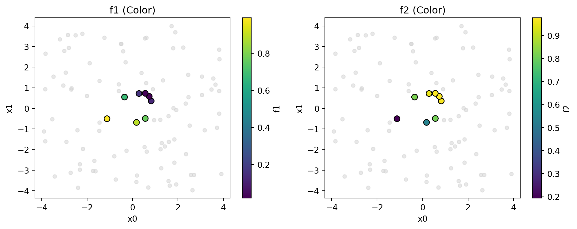
mo_pareto_optx_plot from spotoptim.mo.pareto visualizes Pareto-optimal points in the input space. For each pair of input variables \((x_i, x_j)\) and each objective \(f_k\), it produces a scatter plot where Pareto points are highlighted and colored by their objective value.

import numpy as np
import matplotlib.pyplot as plt
from spotoptim.function import fonseca_fleming
from spotoptim.mo.pareto import mo_pareto_optx_plot

np.random.seed(0)
X = np.random.uniform(-4, 4, size=(100, 2))
Y = fonseca_fleming(X)

mo_pareto_optx_plot(
    X, Y,
    minimize=True,
    feature_names=["x0", "x1"],
    target_names=["f1", "f2"],
)
print("Pareto-optimal input-space visualization complete.")

Pareto-optimal input-space visualization complete.

The module also provides mo_xy_contour and mo_xy_surface for plotting surrogate predictions across objectives. Both accept a list of fitted models together with bounds and produce contour or 3-D surface grids.