plot.visualization.plot_design_points

plot.visualization.plot_design_points(
    X,
    i=0,
    j=1,
    agg='mean',
    show=True,
    **kwargs,
)

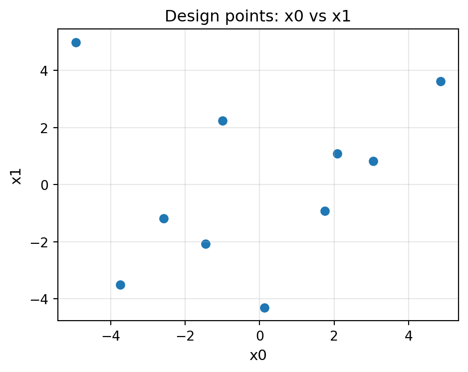
Plot design points projected onto two selected dimensions.

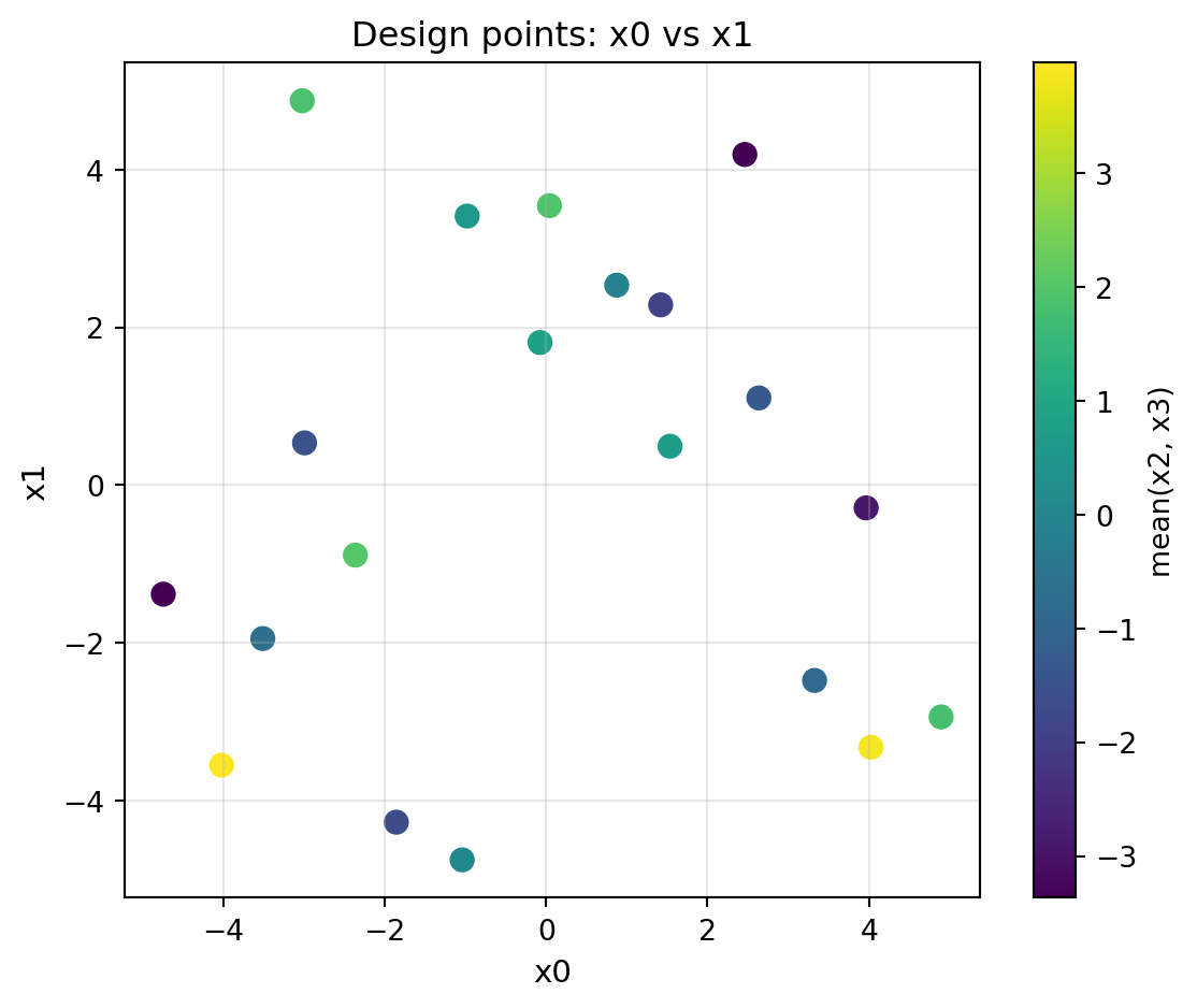
Displays a scatter plot of design points using dimensions i and j as the axes. When X has more than two dimensions, all remaining dimensions (≠ i and ≠ j) are aggregated per point using the agg function, and the result is used to colour the markers.

Parameters

Name	Type	Description	Default
X	np.ndarray	Design matrix of shape `(n_samples, n_dim)`. Each row is one design point.	required
i	int	Index of the dimension to plot on the x-axis. Defaults to `0`.	`0`
j	int	Index of the dimension to plot on the y-axis. Defaults to `1`. Must differ from `i` when `n_dim > 1`.	`1`
agg	str or callable	Aggregation applied to the dimensions that are not plotted (i.e. every column except `i` and `j`). Supported strings: `"mean"`, `"median"`, `"min"`, `"max"`. A callable `f(arr, axis)` is also accepted (e.g. `np.std`). The aggregated value is used as the colour of each marker so that spread across the hidden dimensions is visible at a glance. When `n_dim == 2` this parameter is ignored (no hidden dims). Defaults to `"mean"`.	`'mean'`
show	bool	If `True`, call :func:`matplotlib.pyplot.show` before returning. Set to `False` when running inside tests or scripts that manage display manually. Defaults to `True`.	`True`
**kwargs	object	Additional keyword arguments forwarded to :func:`matplotlib.pyplot.subplots` (e.g. `figsize`) and to :func:`matplotlib.axes.Axes.scatter` (e.g. `s`, `cmap`, `alpha`). `figsize` is intercepted and passed to `subplots`; all other keys go to `scatter`.	`{}`

Returns

Name	Type	Description
	object	matplotlib.figure.Figure: The created figure object. Call
	object	`plt.show()` or `fig.savefig(...)` on the returned object as
	object	needed.

Raises

Name	Type	Description
	ImportError	If matplotlib is not installed.
	ValueError	If `X` is not a 2-D array, has fewer than two columns, or if `i` / `j` are out of range or equal.

Examples

import numpy as np
from spotoptim import SpotOptim
from spotoptim.function import sphere
from spotoptim.plot.visualization import plot_design_points

opt = SpotOptim(
    fun=sphere,
    bounds=[(-5, 5), (-5, 5)],
    n_initial=10,
    seed=42,
)
# Generate a Latin-hypercube initial design (in original scale)
X0 = opt.get_initial_design()

# 2-D design – simple scatter on both dimensions
fig = plot_design_points(X0, i=0, j=1, figsize=(5, 4))

import numpy as np
from spotoptim import SpotOptim
from spotoptim.function import sphere
from spotoptim.plot.visualization import plot_design_points

opt = SpotOptim(
    fun=sphere,
    bounds=[(-5, 5)] * 4,
    n_initial=20,
    seed=42,
)
X0 = opt.get_initial_design()

# 4-D design – colour encodes the mean of the two hidden dimensions
fig = plot_design_points(X0, i=0, j=1, agg="mean", figsize=(6, 5), s=60)