plot.visualization

plot.visualization

Functions

Name Description
plot_design_points Plot design points projected onto two selected dimensions.
plot_important_hyperparameter_contour Plot surrogate contours for all combinations of the top max_imp important parameters.
plot_progress Plot optimization progress showing all evaluations and best-so-far curve.
plot_surrogate Plot the surrogate model for two dimensions.

plot_design_points

plot.visualization.plot_design_points(
    X,
    i=0,
    j=1,
    agg='mean',
    show=True,
    **kwargs,
)

Plot design points projected onto two selected dimensions.

Displays a scatter plot of design points using dimensions i and j as the axes. When X has more than two dimensions, all remaining dimensions (≠ i and ≠ j) are aggregated per point using the agg function, and the result is used to colour the markers.

Parameters

Name Type Description Default
X np.ndarray Design matrix of shape (n_samples, n_dim). Each row is one design point. required
i int Index of the dimension to plot on the x-axis. Defaults to 0. 0
j int Index of the dimension to plot on the y-axis. Defaults to 1. Must differ from i when n_dim > 1. 1
agg str or callable Aggregation applied to the dimensions that are not plotted (i.e. every column except i and j). Supported strings: "mean", "median", "min", "max". A callable f(arr, axis) is also accepted (e.g. np.std). The aggregated value is used as the colour of each marker so that spread across the hidden dimensions is visible at a glance. When n_dim == 2 this parameter is ignored (no hidden dims). Defaults to "mean". 'mean'
show bool If True, call :func:matplotlib.pyplot.show before returning. Set to False when running inside tests or scripts that manage display manually. Defaults to True. True
**kwargs object Additional keyword arguments forwarded to :func:matplotlib.pyplot.subplots (e.g. figsize) and to :func:matplotlib.axes.Axes.scatter (e.g. s, cmap, alpha). figsize is intercepted and passed to subplots; all other keys go to scatter. {}

Returns

Name Type Description
object matplotlib.figure.Figure: The created figure object. Call
object plt.show() or fig.savefig(...) on the returned object as
object needed.

Raises

Name Type Description
ImportError If matplotlib is not installed.
ValueError If X is not a 2-D array, has fewer than two columns, or if i / j are out of range or equal.

Examples

import numpy as np
from spotoptim import SpotOptim
from spotoptim.function import sphere
from spotoptim.plot.visualization import plot_design_points

opt = SpotOptim(
    fun=sphere,
    bounds=[(-5, 5), (-5, 5)],
    n_initial=10,
    seed=42,
)
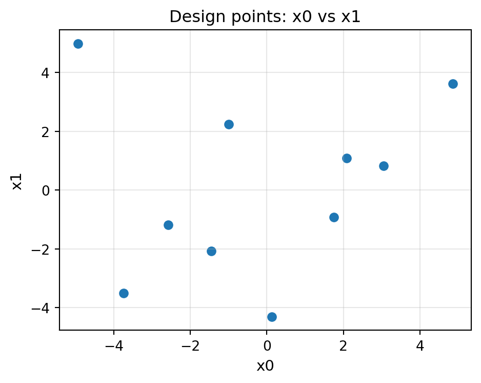
# Generate a Latin-hypercube initial design (in original scale)
X0 = opt.get_initial_design()

# 2-D design – simple scatter on both dimensions
fig = plot_design_points(X0, i=0, j=1, figsize=(5, 4))

import numpy as np
from spotoptim import SpotOptim
from spotoptim.function import sphere
from spotoptim.plot.visualization import plot_design_points

opt = SpotOptim(
    fun=sphere,
    bounds=[(-5, 5)] * 4,
    n_initial=20,
    seed=42,
)
X0 = opt.get_initial_design()

# 4-D design – colour encodes the mean of the two hidden dimensions
fig = plot_design_points(X0, i=0, j=1, agg="mean", figsize=(6, 5), s=60)

plot_important_hyperparameter_contour

plot.visualization.plot_important_hyperparameter_contour(
    optimizer,
    max_imp=3,
    show=True,
    alpha=0.8,
    cmap='jet',
    num=100,
    add_points=True,
    grid_visible=True,
    contour_levels=30,
    figsize=(12, 10),
)

Plot surrogate contours for all combinations of the top max_imp important parameters.

This method identifies the most important parameters using importance scores, then generates surrogate contour plots for all pairwise combinations of these parameters. Factor (categorical) variables are handled by creating discrete grids and displaying factor level names on the axes.

Parameters

Name Type Description Default
optimizer SpotOptimProtocol SpotOptim instance containing optimization data. required
max_imp int Number of most important parameters to visualize. Defaults to 3. For max_imp=3, creates 3 plots: (0,1), (0,2), (1,2). 3
show bool If True, displays plots immediately. Defaults to True. True
alpha float Transparency of 3D surface plots (0=transparent, 1=opaque). Defaults to 0.8. 0.8
cmap str Matplotlib colormap name. Defaults to ‘jet’. 'jet'
num int Number of grid points per dimension. Defaults to 100. For factor variables, uses the number of unique levels instead. 100
add_points bool If True, overlay evaluated points on contour plots. Defaults to True. True
grid_visible bool If True, show grid lines. Defaults to True. True
contour_levels int Number of contour levels. Defaults to 30. 30
figsize tuple of int Figure size in inches (width, height). Defaults to (12, 10). (12, 10)

Raises

Name Type Description
ValueError If optimization hasn’t been run yet or max_imp is invalid.

Examples

import numpy as np
from spotoptim import SpotOptim
from spotoptim.plot.visualization import plot_important_hyperparameter_contour
from spotoptim.function import sphere
# Initialize and run optimizer with enough dimensions (here 4)
opt = SpotOptim(fun=sphere, bounds=[(-5, 5)]*4,
                 max_iter=10, n_initial=5,
                 var_name=['temp', 'pressure', 'velocity', 'acceleration'])
result = opt.optimize()
# Plot contours for top 3 important hyperparameters
plot_important_hyperparameter_contour(opt, max_imp=3, show=False)
Plotting surrogate contours for top 3 most important parameters:
  velocity: importance = 54.93% (type: float)
  acceleration: importance = 30.58% (type: float)
  temp: importance = 8.72% (type: float)

Generating 3 surrogate plots...
  Plotting velocity vs acceleration
  Plotting velocity vs temp
  Plotting acceleration vs temp

plot_progress

plot.visualization.plot_progress(
    optimizer,
    show=True,
    log_y=False,
    figsize=(10, 6),
    ylabel='Objective Value',
    mo=False,
)

Plot optimization progress showing all evaluations and best-so-far curve.

This method visualizes the optimization history, displaying both individual function evaluations and the cumulative best value found. Initial design points are shown as individual scatter points with a light grey background region, while sequential optimization iterations are connected with lines.

Parameters

Name Type Description Default
optimizer SpotOptimProtocol SpotOptim instance containing optimization data. required
show bool Whether to display the plot. Defaults to True. True
log_y bool Whether to use log scale for y-axis. Defaults to False. False
figsize tuple Figure size as (width, height). Defaults to (10, 6). (10, 6)
ylabel str Label for y-axis. Defaults to “Objective Value”. 'Objective Value'
mo bool Whether to plot individual objectives if available. Defaults to False. False

Raises

Name Type Description
ValueError If optimization hasn’t been run yet.
ImportError If matplotlib is not installed.

Examples

import numpy as np
from spotoptim import SpotOptim
from spotoptim.plot.visualization import plot_progress
from spotoptim.function import sphere
opt = SpotOptim(fun=sphere, bounds=[(-5, 5)]*2,
                max_iter=10, n_initial=5, seed=42)
result = opt.optimize()
# Plot optimization progress (linear scale)
plot_progress(opt, log_y=False, show=False)
# Plot with log scale
plot_progress(opt, log_y=True, show=False)

plot_surrogate

plot.visualization.plot_surrogate(
    optimizer,
    i=0,
    j=1,
    show=True,
    alpha=0.8,
    var_name=None,
    cmap='jet',
    num=100,
    vmin=None,
    vmax=None,
    add_points=True,
    grid_visible=True,
    contour_levels=30,
    figsize=(12, 10),
)

Plot the surrogate model for two dimensions.

Creates a 2x2 plot showing: - Top left: 3D surface of predictions - Top right: 3D surface of prediction uncertainty - Bottom left: Contour plot of predictions with evaluated points - Bottom right: Contour plot of prediction uncertainty

Parameters

Name Type Description Default
optimizer SpotOptimProtocol SpotOptim instance containing optimization data and surrogate model. required
i int Index of the first dimension to plot. Defaults to 0. 0
j int Index of the second dimension to plot. Defaults to 1. 1
show bool If True, displays the plot immediately. Defaults to True. True
alpha float Transparency of the 3D surface plots (0=transparent, 1=opaque). Defaults to 0.8. 0.8
var_name list of str Names for each dimension. If None, uses instance var_name. Defaults to None. None
cmap str Matplotlib colormap name. Defaults to ‘jet’. 'jet'
num int Number of grid points per dimension for mesh grid. Defaults to 100. 100
vmin float Minimum value for color scale. If None, determined from data. Defaults to None. None
vmax float Maximum value for color scale. If None, determined from data. Defaults to None. None
add_points bool If True, overlay evaluated points on contour plots. Defaults to True. True
grid_visible bool If True, show grid lines on contour plots. Defaults to True. True
contour_levels int Number of contour levels. Defaults to 30. 30
figsize tuple of int Figure size in inches (width, height). Defaults to (12, 10). (12, 10)

Raises

Name Type Description
ValueError If optimization hasn’t been run yet, or if i, j are invalid.
ImportError If matplotlib is not installed.

Examples

import numpy as np
from spotoptim import SpotOptim
from spotoptim.plot.visualization import plot_surrogate
from spotoptim.function import sphere
opt = SpotOptim(fun=sphere,
                bounds=[(-5, 5), (-5, 5)],
                max_iter=10,
                n_initial=5,
                var_name=['x1', 'x2'])
result = opt.optimize()
# Plot surrogate model for dimensions 0 and 1
plot_surrogate(opt, i=0, j=1, show=False)