MAX_TIME = 1
INIT_SIZE = 5
PREFIX="025RIVER"
K = 0.121 river Hyperparameter Tuning: Mondrian Tree Regressor with Friedman Drift Data
This chapter demonstrates hyperparameter tuning for river’s Mondrian Tree Regressor with the Friedman drift data set [SOURCE]. The Mondrian Tree Regressor is a regression tree, i.e., it predicts a real value for each sample.
21.1 Setup
Before we consider the detailed experimental setup, we select the parameters that affect run time, initial design size, size of the data set, and the experiment name.
MAX_TIME: The maximum run time in seconds for the hyperparameter tuning process.INIT_SIZE: The initial design size for the hyperparameter tuning process.PREFIX: The prefix for the experiment name.K: The factor that determines the number of samples in the data set.
Caution: Run time and initial design size should be increased for real experiments
MAX_TIMEis set to one minute for demonstration purposes. For real experiments, this should be increased to at least 1 hour.INIT_SIZEis set to 5 for demonstration purposes. For real experiments, this should be increased to at least 10.Kis the multiplier for the number of samples. If it is set to 1, then100_000samples are taken. It is set to 0.1 for demonstration purposes. For real experiments, this should be increased to at least 1.
- This notebook exemplifies hyperparameter tuning with SPOT (spotPython and spotRiver).
- The hyperparameter software SPOT is available in Python. It was developed in R (statistical programming language), see Open Access book “Hyperparameter Tuning for Machine and Deep Learning with R - A Practical Guide”, available here: https://link.springer.com/book/10.1007/978-981-19-5170-1.
- This notebook demonstrates hyperparameter tuning for
river. It is based on the notebook “Incremental decision trees in river: the Hoeffding Tree case”, see: https://riverml.xyz/0.15.0/recipes/on-hoeffding-trees/#42-regression-tree-splitters. - Here we will use the river
AMFRegressorfunctions, see: https://riverml.xyz/0.19.0/api/forest/AMFRegressor/.
21.2 Initialization of the fun_control Dictionary
spotPython supports the visualization of the hyperparameter tuning process with TensorBoard. The following example shows how to use TensorBoard with spotPython.
First, we define an “experiment name” to identify the hyperparameter tuning process. The experiment name is also used to create a directory for the TensorBoard files.
from spotPython.utils.init import fun_control_init
fun_control = fun_control_init(
    PREFIX=PREFIX,
    TENSORBOARD_CLEAN=True,
    max_time=MAX_TIME,
    fun_evals=inf,
    tolerance_x=np.sqrt(np.spacing(1)))
Moving TENSORBOARD_PATH: runs/ to TENSORBOARD_PATH_OLD: runs_OLD/runs_2024_04_22_00_38_43
Created spot_tensorboard_path: runs/spot_logs/025RIVER_maans14_2024-04-22_00-38-43 for SummaryWriter()
Tip: TensorBoard
- Since the
spot_tensorboard_pathargument is notNone, which is the default,spotPythonwill log the optimization process in the TensorBoard folder. - Section 21.8.3 describes how to start TensorBoard and access the TensorBoard dashboard.
- The
TENSORBOARD_CLEANargument is set toTrueto archive the TensorBoard folder if it already exists. This is useful if you want to start a hyperparameter tuning process from scratch. If you want to continue a hyperparameter tuning process, setTENSORBOARD_CLEANtoFalse. Then the TensorBoard folder will not be archived and the old and new TensorBoard files will shown in the TensorBoard dashboard.
21.3 Load Data: The Friedman Drift Data
We will use the Friedman synthetic dataset with concept drifts [SOURCE]. Each observation is composed of ten features. Each feature value is sampled uniformly in [0, 1]. Only the first five features are relevant. The target is defined by different functions depending on the type of the drift. Global Recurring Abrupt drift will be used, i.e., the concept drift appears over the whole instance space. There are two points of concept drift. At the second point of drift the old concept reoccurs.
The following parameters are used to generate and handle the data set:
- horizon: The prediction horizon in hours.
- n_samples: The number of samples in the data set.
- p_1: The position of the first concept drift.
- p_2: The position of the second concept drift.
- position: The position of the concept drifts.
- n_train: The number of samples used for training.
horizon = 7*24
n_samples = int(K*100_000)
p_1 = int(K*25_000)
p_2 = int(K*50_000)
position=(p_1, p_2)
n_train = 1_000
from river.datasets import synth
import pandas as pd
dataset = synth.FriedmanDrift(
drift_type='gra',
position=position,
seed=123
)- We will use
spotRiver’sconvert_to_dffunction [SOURCE] to convert theriverdata set to apandasdata frame.
from spotRiver.utils.data_conversion import convert_to_df
target_column = "y"
df = convert_to_df(dataset, target_column=target_column, n_total=n_samples)- Add column names x1 until x10 to the first 10 columns of the dataframe and the column name y to the last column of the dataframe.
- Then split the data frame into a training and test data set. The train and test data sets are stored in the
fun_controldictionary.
from spotPython.hyperparameters.values import set_control_key_value
df.columns = [f"x{i}" for i in range(1, 11)] + ["y"]
set_control_key_value(control_dict=fun_control,
                        key="train",
                        value=df[:n_train],
                        replace=True)
set_control_key_value(fun_control, "test", df[n_train:], True)
set_control_key_value(fun_control, "n_samples", n_samples, replace=True)
set_control_key_value(fun_control, "target_column", target_column, replace=True)
21.4 Specification of the Preprocessing Model
- We use the
StandardScaler[SOURCE] fromriveras the preprocessing model. TheStandardScaleris used to standardize the data set, i.e., it has zero mean and unit variance.
from river import preprocessing
prep_model = preprocessing.StandardScaler()
set_control_key_value(fun_control, "prep_model", prep_model, replace=True)
21.5 SelectSelect Model (algorithm) and core_model_hyper_dict
spotPython hyperparameter tuning approach uses two components:
- a model (class) and
- an associated hyperparameter dictionary.
The corresponding hyperparameters are loaded from the associated dictionary, which is stored as a JSON file [SOURCE]. The JSON file contains hyperparameter type information, names, and bounds.
The method add_core_model_to_fun_control adds the model and the hyperparameter dictionary to the fun_control dictionary.
Alternatively, you can load a local hyper_dict. Simply set river_hyper_dict.json as the filename. If filenameis set to None, which is the default, the hyper_dict [SOURCE] is loaded from the spotRiver package.
from river.forest import AMFRegressor
from spotRiver.hyperdict.river_hyper_dict import RiverHyperDict
from spotPython.hyperparameters.values import add_core_model_to_fun_control
add_core_model_to_fun_control(core_model=AMFRegressor,
                              fun_control=fun_control,
                              hyper_dict=RiverHyperDict,
                              filename=None)
21.6 Modify hyper_dict Hyperparameters for the Selected Algorithm aka core_model
After the core_model and the core_model_hyper_dict are added to the fun_control dictionary, the hyperparameter tuning can be started. However, in some settings, the user wants to modify the hyperparameters of the core_model_hyper_dict. This can be done with the modify_hyper_parameter_bounds and modify_hyper_parameter_levels functions [SOURCE].
The following code shows how hyperparameter of type numeric and integer (boolean) can be modified. The modify_hyper_parameter_bounds function is used to modify the bounds of the hyperparameter delta and merit_preprune. Similar option exists for the modify_hyper_parameter_levels function to modify the levels of categorical hyperparameters.
# from spotPython.hyperparameters.values import modify_hyper_parameter_bounds
# modify_hyper_parameter_bounds(fun_control, "n_estimators", bounds=[2,100])

from spotPython.hyperparameters.values import set_control_hyperparameter_value
set_control_hyperparameter_value(fun_control, "n_estimators", [2, 100])
Setting hyperparameter n_estimators to value [2, 100].
Variable type is int.
Core type is None.
Calling modify_hyper_parameter_bounds().::: {.callout-note} #### Note: Active and Inactive Hyperparameters Hyperparameters can be excluded from the tuning procedure by selecting identical values for the lower and upper bounds.
from spotPython.utils.eda import gen_design_table
print(gen_design_table(fun_control))
| name | type | default | lower | upper | transform |
|-----------------|--------|-----------|---------|---------|-------------|
| n_estimators | int | 10 | 2 | 100 | None |
| step | float | 1 | 0.1 | 10 | None |
| use_aggregation | factor | 1 | 0 | 1 | None |21.7 Selection of the Objective (Loss) Function
The metric_sklearn is used for the sklearn based evaluation via eval_oml_horizon [SOURCE]. Here we use the mean_absolute_error [SOURCE] as the objective function.
Note: Additional metrics
spotRiver also supports additional metrics. For example, the metric_river is used for the river based evaluation via eval_oml_iter_progressive [SOURCE]. The metric_river is implemented to simulate the behaviour of the “original” river metrics.
spotRiver provides information about the model’ s score (metric), memory, and time. The hyperparamter tuner requires a single objective. Therefore, a weighted sum of the metric, memory, and time is computed. The weights are defined in the weights array.
Note: Weights
The weights provide a flexible way to define specific requirements, e.g., if the memory is more important than the time, the weight for the memory can be increased.
The oml_grace_period defines the number of observations that are used for the initial training of the model. The step defines the iteration number at which to yield results. This only takes into account the predictions, and not the training steps. The weight_coeff defines a multiplier for the results: results are multiplied by (step/n_steps)**weight_coeff, where n_steps is the total number of iterations. Results from the beginning have a lower weight than results from the end if weight_coeff > 1. If weight_coeff == 0, all results have equal weight. Note, that the weight_coeff is only used internally for the tuner and does not affect the results that are used for the evaluation or comparisons.
import numpy as np
from sklearn.metrics import mean_absolute_error

weights = np.array([1, 1/1000, 1/1000])*10_000.0
oml_grace_period = 2
step = 100
weight_coeff = 1.0

# fun_control.update({
#                "horizon": horizon,
#                "oml_grace_period": oml_grace_period,
#                "weights": weights,
#                "step": step,
#                "weight_coeff": weight_coeff,
#                "metric_sklearn": mean_absolute_error
#                })
set_control_key_value(control_dict=fun_control,
                        key="horizon",
                        value=horizon,
                        replace=True)
set_control_key_value(fun_control, "oml_grace_period", oml_grace_period, True)
set_control_key_value(fun_control, "weights", weights, True)
set_control_key_value(fun_control, "step", step, True)
set_control_key_value(fun_control, "weight_coeff", weight_coeff, True)
set_control_key_value(fun_control, "metric_sklearn", mean_absolute_error, True)
21.8 Calling the SPOT Function
21.8.1 The Objective Function
The objective function fun_oml_horizon [SOURCE] is selected next.
from spotRiver.fun.hyperriver import HyperRiver
fun = HyperRiver().fun_oml_horizon
The following code snippet shows how to get the default hyperparameters as an array, so that they can be passed to the Spot function.
from spotPython.hyperparameters.values import get_default_hyperparameters_as_array
X_start = get_default_hyperparameters_as_array(fun_control)
21.8.2 Run the Spot Optimizer
The class Spot [SOURCE] is the hyperparameter tuning workhorse. It is initialized with the following parameters:
fun: the objective functionfun_control: the dictionary with the control parameters for the objective functiondesign: the experimental designdesign_control: the dictionary with the control parameters for the experimental designsurrogate: the surrogate modelsurrogate_control: the dictionary with the control parameters for the surrogate modeloptimizer: the optimizeroptimizer_control: the dictionary with the control parameters for the optimizer
Note: Total run time
The total run time may exceed the specified max_time, because the initial design (here: init_size = INIT_SIZE as specified above) is always evaluated, even if this takes longer than max_time.
from spotPython.utils.init import design_control_init, surrogate_control_init
design_control = design_control_init()
set_control_key_value(control_dict=design_control,
                        key="init_size",
                        value=INIT_SIZE,
                        replace=True)

surrogate_control = surrogate_control_init(noise=True,
                                           n_theta=2)
from spotPython.spot import spot
spot_tuner = spot.Spot(fun=fun,
fun_control=fun_control,
design_control=design_control,
surrogate_control=surrogate_control)
spot_tuner.run(X_start=X_start)spotPython tuning: 26517.73333435744 [##########] 100.00% Done...
{'CHECKPOINT_PATH': 'runs/saved_models/',
'DATASET_PATH': 'data/',
'PREFIX': '025RIVER',
'RESULTS_PATH': 'results/',
'TENSORBOARD_PATH': 'runs/',
'_L_in': None,
'_L_out': None,
'_torchmetric': None,
'accelerator': 'auto',
'converters': None,
'core_model': <class 'river.forest.aggregated_mondrian_forest.AMFRegressor'>,
'core_model_hyper_dict': {'n_estimators': {'default': 10,
'lower': 2,
'transform': 'None',
'type': 'int',
'upper': 100},
'step': {'default': 1.0,
'lower': 0.1,
'transform': 'None',
'type': 'float',
'upper': 10},
'use_aggregation': {'core_model_parameter_type': 'bool',
'default': 1,
'levels': [0, 1],
'lower': 0,
'transform': 'None',
'type': 'factor',
'upper': 1}},
'core_model_hyper_dict_default': {'n_estimators': {'default': 10,
'lower': 2,
'transform': 'None',
'type': 'int',
'upper': 1000},
'step': {'default': 1.0,
'lower': 0.1,
'transform': 'None',
'type': 'float',
'upper': 10},
'use_aggregation': {'core_model_parameter_type': 'bool',
'default': 1,
'levels': [0, 1],
'lower': 0,
'transform': 'None',
'type': 'factor',
'upper': 1}},
'core_model_name': None,
'counter': 7,
'data': None,
'data_dir': './data',
'data_module': None,
'data_set': None,
'data_set_name': None,
'db_dict_name': None,
'design': None,
'device': None,
'devices': 1,
'enable_progress_bar': False,
'eval': None,
'fun_evals': inf,
'fun_repeats': 1,
'horizon': 168,
'infill_criterion': 'y',
'k_folds': 3,
'log_graph': False,
'log_level': 50,
'loss_function': None,
'lower': array([2. , 0.1, 0. ]),
'max_surrogate_points': 30,
'max_time': 1,
'metric_params': {},
'metric_river': None,
'metric_sklearn': <function mean_absolute_error at 0x3bc7d72e0>,
'metric_sklearn_name': None,
'metric_torch': None,
'model_dict': {},
'n_points': 1,
'n_samples': 10000,
'n_total': None,
'noise': False,
'num_workers': 0,
'ocba_delta': 0,
'oml_grace_period': 2,
'optimizer': None,
'path': None,
'prep_model': StandardScaler (
with_std=True
),
'prep_model_name': None,
'progress_file': None,
'save_model': False,
'scenario': None,
'seed': 123,
'show_batch_interval': 1000000,
'show_models': False,
'show_progress': True,
'shuffle': None,
'sigma': 0.0,
'spot_tensorboard_path': 'runs/spot_logs/025RIVER_maans14_2024-04-22_00-38-43',
'spot_writer': <torch.utils.tensorboard.writer.SummaryWriter object at 0x3ba448f50>,
'step': 100,
'target_column': 'y',
'target_type': None,
'task': None,
'test': x1 x2 x3 x4 x5 x6 x7 \
1000 0.149257 0.456455 0.086002 0.012030 0.743199 0.555736 0.233676
1001 0.319370 0.286723 0.281127 0.647570 0.697423 0.474675 0.788735
1002 0.339058 0.052272 0.096132 0.449870 0.732686 0.249310 0.095512
1003 0.223965 0.080771 0.532323 0.820374 0.662628 0.616938 0.195786
1004 0.007170 0.893475 0.408799 0.394976 0.990258 0.925658 0.256272
... ... ... ... ... ... ... ...
9995 0.707825 0.823946 0.482666 0.839029 0.073890 0.074298 0.397132
9996 0.033073 0.995334 0.888897 0.339522 0.838881 0.862215 0.045144
9997 0.357023 0.305839 0.185412 0.954059 0.361154 0.834810 0.516624
9998 0.347719 0.079667 0.981140 0.656389 0.931914 0.955769 0.620668
9999 0.310359 0.563592 0.258083 0.502411 0.159050 0.278782 0.296032
x8 x9 x10 y
1000 0.319511 0.865121 0.104190 9.639799
1001 0.698887 0.767774 0.217209 11.859974
1002 0.855869 0.413789 0.487099 11.761361
1003 0.419200 0.656080 0.172583 12.168891
1004 0.447393 0.564091 0.868190 12.685521
... ... ... ... ...
9995 0.106350 0.489138 0.621020 18.611413
9996 0.677220 0.138391 0.371764 12.492723
9997 0.723574 0.033693 0.884783 17.682427
9998 0.690811 0.037812 0.293507 16.380985
9999 0.246599 0.518025 0.620904 13.135314
[9000 rows x 11 columns],
'test_seed': 1234,
'test_size': 0.4,
'tolerance_x': 1.4901161193847656e-08,
'train': x1 x2 x3 x4 x5 x6 x7 \
0 0.052364 0.087187 0.407242 0.107700 0.901199 0.038154 0.536202
1 0.245163 0.001671 0.436276 0.087613 0.597599 0.069877 0.315459
2 0.142175 0.790072 0.021236 0.911151 0.573408 0.265322 0.837838
3 0.527075 0.809339 0.315263 0.398238 0.769279 0.512752 0.684837
4 0.486136 0.668470 0.374522 0.031841 0.754173 0.181465 0.820190
.. ... ... ... ... ... ... ...
995 0.054258 0.151721 0.743083 0.802598 0.078008 0.106518 0.613012
996 0.891570 0.396470 0.776985 0.086130 0.588280 0.760256 0.260412
997 0.840034 0.318170 0.923870 0.733199 0.715419 0.805433 0.606878
998 0.935949 0.987038 0.629630 0.360930 0.856310 0.330804 0.836771
999 0.125361 0.059499 0.518353 0.705182 0.762343 0.347013 0.725256
x8 x9 x10 y
0 0.332198 0.852087 0.159662 5.428947
1 0.448322 0.905399 0.092765 4.727526
2 0.768795 0.343462 0.801497 20.385826
3 0.638353 0.666658 0.890099 19.566743
4 0.913646 0.658074 0.170127 12.412629
.. ... ... ... ...
995 0.525063 0.911144 0.870062 11.913435
996 0.016439 0.988105 0.910124 14.573648
997 0.584725 0.735601 0.228933 22.611338
998 0.851467 0.259093 0.438976 10.898222
999 0.836309 0.316067 0.002152 11.526148
[1000 rows x 11 columns],
'upper': array([1000, 10, 1]),
'var_name': ['n_estimators', 'step', 'use_aggregation'],
'var_type': ['int', 'float', 'factor'],
'verbosity': 0,
'weight_coeff': 1.0,
'weights': array([10000., 10., 10.]),
'weights_entry': None}<spotPython.spot.spot.Spot at 0x3bd5d04d0>21.8.3 TensorBoard
Now we can start TensorBoard in the background with the following command, where ./runs is the default directory for the TensorBoard log files:
tensorboard --logdir="./runs"
Tip: TENSORBOARD_PATH
The TensorBoard path can be printed with the following command:
from spotPython.utils.init import get_tensorboard_path
get_tensorboard_path(fun_control)'runs/'We can access the TensorBoard web server with the following URL:
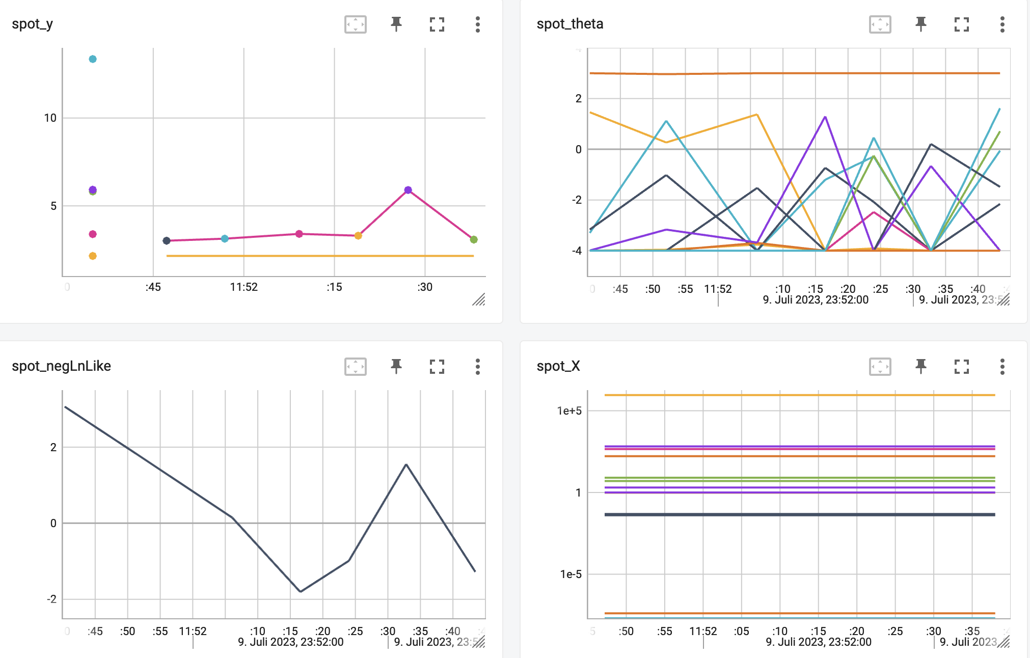
http://localhost:6006/The TensorBoard plot illustrates how spotPython can be used as a microscope for the internal mechanisms of the surrogate-based optimization process. Here, one important parameter, the learning rate \(\theta\) of the Kriging surrogate [SOURCE] is plotted against the number of optimization steps.
21.8.4 Results
After the hyperparameter tuning run is finished, the results can be saved and reloaded with the following commands:
from spotPython.utils.file import save_pickle,  load_pickle
from spotPython.utils.init import get_experiment_name
experiment_name = get_experiment_name(PREFIX)
SAVE_AND_LOAD = False
if SAVE_AND_LOAD == True:
    save_pickle(spot_tuner, experiment_name)
    spot_tuner = load_pickle(experiment_name)
After the hyperparameter tuning run is finished, the progress of the hyperparameter tuning can be visualized. The black points represent the performace values (score or metric) of hyperparameter configurations from the initial design, whereas the red points represents the hyperparameter configurations found by the surrogate model based optimization.
spot_tuner.plot_progress(log_y=True, filename="./figures/" + experiment_name+"_progress.pdf")
Results can also be printed in tabular form.
print(gen_design_table(fun_control=fun_control, spot=spot_tuner))| name | type | default | lower | upper | tuned | transform | importance | stars |
|-----------------|--------|-----------|---------|---------|------------------|-------------|--------------|---------|
| n_estimators | int | 10.0 | 2.0 | 100 | 57.0 | None | 100.00 | *** |
| step | float | 1.0 | 0.1 | 10 | 3.71170631585164 | None | 70.85 | ** |
| use_aggregation | factor | 1.0 | 0.0 | 1 | 1.0 | None | 12.24 | * |A histogram can be used to visualize the most important hyperparameters.
spot_tuner.plot_importance(threshold=0.0025, filename="./figures/" + experiment_name+"_importance.pdf")
21.9 The Larger Data Set
After the hyperparameter were tuned on a small data set, we can now apply the hyperparameter configuration to a larger data set. The following code snippet shows how to generate the larger data set.
Caution: Increased Friedman-Drift Data Set
- The Friedman-Drift Data Set is increased by a factor of two to show the transferability of the hyperparameter tuning results.
- Larger values of
Klead to a longer run time.
K = 0.2
n_samples = int(K*100_000)
p_1 = int(K*25_000)
p_2 = int(K*50_000)
position=(p_1, p_2)
dataset = synth.FriedmanDrift(
drift_type='gra',
position=position,
seed=123
)The larger data set is converted to a Pandas data frame and passed to the fun_control dictionary.
df = convert_to_df(dataset, target_column=target_column, n_total=n_samples)
df.columns = [f"x{i}" for i in range(1, 11)] + ["y"]
# fun_control.update({"train": df[:n_train],
#                     "test": df[n_train:],
#                     "n_samples": n_samples,
#                     "target_column": target_column})
set_control_key_value(fun_control, "train", df[:n_train], True)
set_control_key_value(fun_control, "test", df[n_train:], True)
set_control_key_value(fun_control, "n_samples", n_samples, True)
set_control_key_value(fun_control, "target_column", target_column, True)
21.10 Get Default Hyperparameters
The default hyperparameters, whihc will be used for a comparion with the tuned hyperparameters, can be obtained with the following commands:
from spotPython.hyperparameters.values import get_one_core_model_from_X
from spotPython.hyperparameters.values import get_default_hyperparameters_as_array
X_start = get_default_hyperparameters_as_array(fun_control)
model_default = get_one_core_model_from_X(X_start, fun_control, default=True)
Note:
spotPython tunes numpy arrays
spotPythontunes numpy arrays, i.e., the hyperparameters are stored in a numpy array.
The model with the default hyperparameters can be trained and evaluated with the following commands:
from spotRiver.evaluation.eval_bml import eval_oml_horizon

df_eval_default, df_true_default = eval_oml_horizon(
                    model=model_default,
                    train=fun_control["train"],
                    test=fun_control["test"],
                    target_column=fun_control["target_column"],
                    horizon=fun_control["horizon"],
                    oml_grace_period=fun_control["oml_grace_period"],
                    metric=fun_control["metric_sklearn"],
                )
The three performance criteria, i.e., scaoe (metric), runtime, and memory consumption, can be visualized with the following commands:
from spotRiver.evaluation.eval_bml import plot_bml_oml_horizon_metrics, plot_bml_oml_horizon_predictions
df_labels=["default"]
plot_bml_oml_horizon_metrics(df_eval = [df_eval_default], log_y=False, df_labels=df_labels, metric=fun_control["metric_sklearn"])
21.10.1 Show Predictions
- Select a subset of the data set for the visualization of the predictions:
- We use the mean, \(m\), of the data set as the center of the visualization.
- We use 100 data points, i.e., \(m \pm 50\) as the visualization window.
m = fun_control["test"].shape[0]
a = int(m/2)-50
b = int(m/2)
plot_bml_oml_horizon_predictions(df_true = [df_true_default[a:b]], target_column=target_column, df_labels=df_labels)
21.11 Get SPOT Results
In a similar way, we can obtain the hyperparameters found by spotPython.
from spotPython.hyperparameters.values import get_one_core_model_from_X
X = spot_tuner.to_all_dim(spot_tuner.min_X.reshape(1,-1))
model_spot = get_one_core_model_from_X(X, fun_control)
df_eval_spot, df_true_spot = eval_oml_horizon(
model=model_spot,
train=fun_control["train"],
test=fun_control["test"],
target_column=fun_control["target_column"],
horizon=fun_control["horizon"],
oml_grace_period=fun_control["oml_grace_period"],
metric=fun_control["metric_sklearn"],
)df_labels=["default", "spot"]
plot_bml_oml_horizon_metrics(df_eval = [df_eval_default, df_eval_spot], log_y=False, df_labels=df_labels, metric=fun_control["metric_sklearn"], filename="./figures/" + experiment_name+"_metrics.pdf")
plot_bml_oml_horizon_predictions(df_true = [df_true_default[a:b], df_true_spot[a:b]], target_column=target_column, df_labels=df_labels, filename="./figures/" + experiment_name+"_predictions.pdf")
from spotPython.plot.validation import plot_actual_vs_predicted
plot_actual_vs_predicted(y_test=df_true_default[target_column], y_pred=df_true_default["Prediction"], title="Default")
plot_actual_vs_predicted(y_test=df_true_spot[target_column], y_pred=df_true_spot["Prediction"], title="SPOT")

21.12 Detailed Hyperparameter Plots
filename = "./figures/" + experiment_name
spot_tuner.plot_important_hyperparameter_contour(filename=filename)
n_estimators: 100.0
step: 70.84616962601444
use_aggregation: 12.242874151228666
impo: [['n_estimators', 100.0], ['step', 70.84616962601444], ['use_aggregation', 12.242874151228666]]
indices: [0, 1, 2]
indices after max_imp selection: [0, 1, 2]


21.13 Parallel Coordinates Plots
spot_tuner.parallel_plot()21.14 Plot all Combinations of Hyperparameters
- Warning: this may take a while.
PLOT_ALL = False
if PLOT_ALL:
    n = spot_tuner.k
    for i in range(n-1):
        for j in range(i+1, n):
            spot_tuner.plot_contour(i=i, j=j, min_z=min_z, max_z = max_z)