19 Simplifying Hyperparameter Tuning in Online Machine Learning—The spotRiverGUI
19.1 Introduction
Batch Machine Learning (BML) often encounters limitations when processing substantial volumes of streaming data (Keller-McNulty 2004; Gaber, Zaslavsky, and Krishnaswamy 2005; Aggarwal 2007). These limitations become particularly evident in terms of available memory, managing drift in data streams (Bifet and Gavaldà 2007, 2009; Gama et al. 2004; Bartz-Beielstein 2024c), and processing novel, unclassified data (Bifet 2010), (Dredze, Oates, and Piatko 2010). As a solution, Online Machine Learning (OML) serves as an effective alternative to BML, adeptly addressing these constraints. OML’s ability to sequentially process data proves especially beneficial for handling data streams (Bifet et al. 2010a; Masud et al. 2011; Gama, Sebastião, and Rodrigues 2013; Putatunda 2021; Bartz-Beielstein and Hans 2024).
The Online Machine Learning (OML) methods provided by software packages such as river (Montiel et al. 2021) or MOA (Bifet et al. 2010b) require the specification of many hyperparameters. To give an example, Hoeffding trees (Hoeglinger and Pears 2007), which are very popular in OML, offer a variety of “splitters” to generate subtrees. There are also several methods to limit the tree size, ensuring time and memory requirements remain manageable. Given the multitude of parameters, manually searching for the optimal hyperparameter setting can be a daunting and often futile task due to the complexity of possible combinations. This article elucidates how automatic hyperparameter optimization, or “tuning”, can be achieved. Beyond optimizing the OML process, Hyperparameter Tuning (HPT) executed with the Sequential Parameter Optimization Toolbox (SPOT) enhances the explainability and interpretability of OML procedures. This can result in a more efficient, resource-conserving algorithm, contributing to the concept of “Green AI”.
Note: This document refers to spotRiverGUI version 0.0.26 which was released on Feb 18, 2024 on GitHub, see: https://github.com/sequential-parameter-optimization/spotGUI/tree/main. The GUI is under active development and new features will be added soon.
This article describes the spotRiverGUI, which is a graphical user interface for the spotRiver package. The GUI allows the user to select the task, the data set, the preprocessing model, the metric, and the online machine learning model. The user can specify the experiment duration, the initial design, and the evaluation options. The GUI provides information about the data set and allows the user to save and load experiments. It also starts and stops a tensorboard process to observe the tuning online and provides an analysis of the hyperparameter tuning process. The spotRiverGUI releases the user from the burden of manually searching for the optimal hyperparameter setting. After providing the data, users can compare different OML algorithms from the powerful river package in a convenient way and tune the selected algorithm very efficiently.
This article is structured as follows:
Section 19.2 describes how to install the software. It also explains how the spotRiverGUI can be started. Section 19.3 describes the binary classification task and the options available in the spotRiverGUI. Section 19.4 provides information about the planned regression task. Section 19.5 describes how the data can be visualized in the spotRiverGUI. Section 19.6 provides information about saving and loading experiments. Section 19.7 describes how to start an experiment and how the associated tensorboard process can be started and stopped. Section 19.8 provides information about the analysis of the results from the hyperparameter tuning process. Section 19.9 concludes the article and provides an outlook.
19.2 Installation and Starting
19.2.1 Installation
We strongly recommend using a virtual environment for the installation of the river, spotRiver, build and spotRiverGUI packages.
Miniforge, which holds the minimal installers for Conda, is a good starting point. Please follow the instructions on https://github.com/conda-forge/miniforge. Using Conda, the following commands can be used to create a virtual environment (Python 3.11 is recommended):
>> conda create -n myenv python=3.11
>> conda activate myenv
Now the river and spotRiver packages can be installed:
>> (myenv) pip install river spotRiver buildAlthough the spotGUI package is available on PyPI, we recommend an installation from the GitHub repository https://github.com/sequential-parameter-optimization/spotGUI, because the spotGUI package is under active development and new features will be added soon. The installation from the GitHub repository is done by executing the following command:
>> (myenv) git clone git@github.com:sequential-parameter-optimization/spotGUI.gitBuilding the spotGUI package is done by executing the following command:
>> (myenv) cd spotGUI
>> (myenv) python -m build
Now the spotRiverGUI package can be installed:
>> (myenv) pip install dist/spotGUI-0.0.26.tar.gz19.2.2 Starting the GUI
The GUI can be started by executing the spotRiverGUI.py file in the spotGUI/spotRiverGUI directory. Change to the spotRiverGUI directory and start the GUI:
>> (myenv) cd spotGUI/spotRiverGUI
>> (myenv) python spotRiverGUI.py
The GUI window will open, as shown in Figure 19.1.
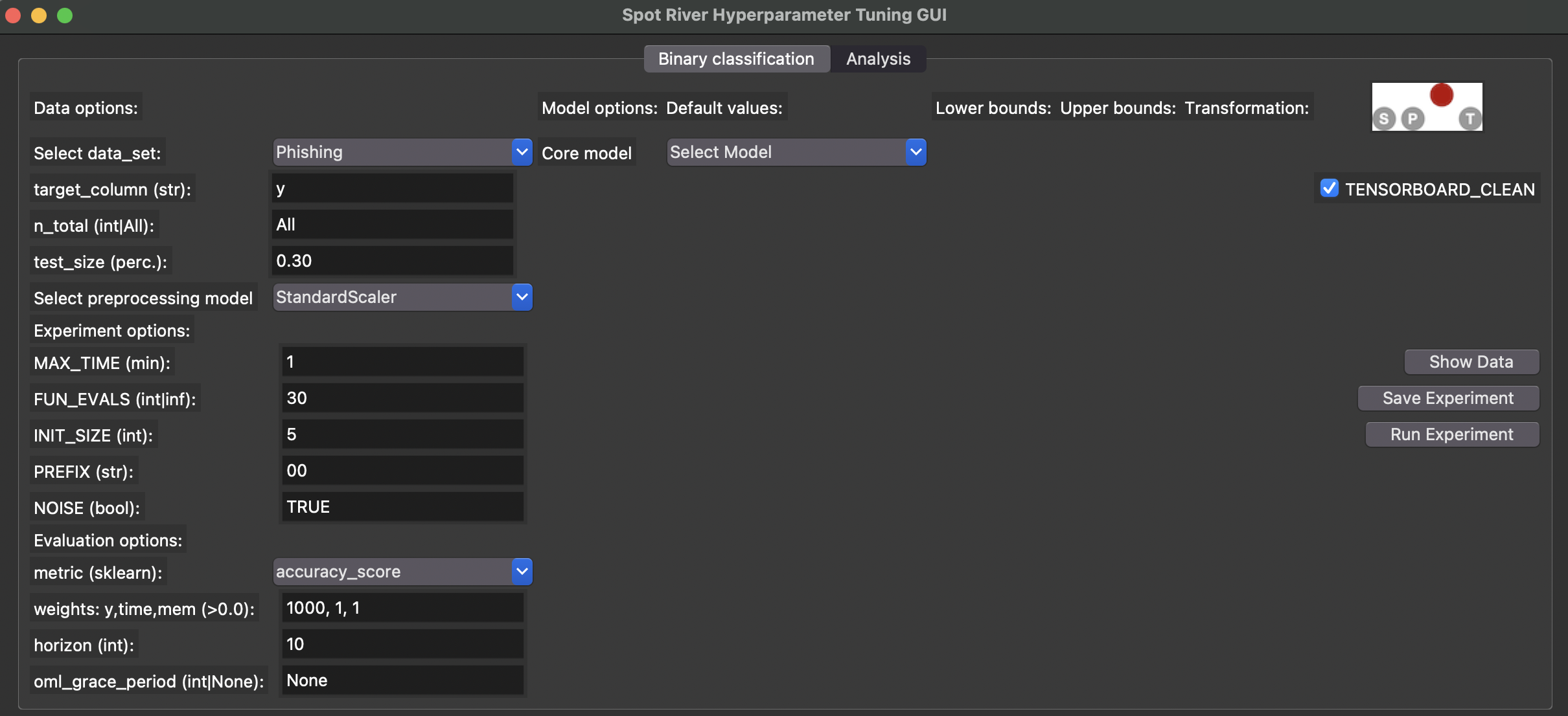
After the GUI window has opened, the user can select the task. Currently, Binary Classification is available. Further tasks like Regression will be available soon.
Depending on the task, the user can select the data set, the preprocessing model, the metric, and the online machine learning model.
19.3 Binary Classification
19.3.1 Binary Classification Options
If the Binary Classification task is selected, the user can select pre-specified data sets from the Data drop-down menu.
19.3.1.1 River Data Sets
The following data sets from the river package are available (the descriptions are taken from the river package):
Bananas: An artificial dataset where instances belongs to several clusters with a banana shape.There are two attributes that correspond to the x and y axis, respectively. More: https://riverml.xyz/dev/api/datasets/Bananas/.CreditCard: Credit card frauds. The datasets contains transactions made by credit cards in September 2013 by European cardholders. Feature ‘Class’ is the response variable and it takes value 1 in case of fraud and 0 otherwise. More: https://riverml.xyz/dev/api/datasets/CreditCard/.Elec2: Electricity prices in New South Wales. This is a binary classification task, where the goal is to predict if the price of electricity will go up or down. This data was collected from the Australian New South Wales Electricity Market. In this market, prices are not fixed and are affected by demand and supply of the market. They are set every five minutes. Electricity transfers to/from the neighboring state of Victoria were done to alleviate fluctuations. More: https://riverml.xyz/dev/api/datasets/Elec2/.Higgs: The data has been produced using Monte Carlo simulations. The first 21 features (columns 2-22) are kinematic properties measured by the particle detectors in the accelerator. The last seven features are functions of the first 21 features; these are high-level features derived by physicists to help discriminate between the two classes. More: https://riverml.xyz/dev/api/datasets/Higgs/.HTTP: HTTP dataset of the KDD 1999 cup. The goal is to predict whether or not an HTTP connection is anomalous or not. The dataset only contains 2,211 (0.4%) positive labels. More: https://riverml.xyz/dev/api/datasets/HTTP/.Phishing: Phishing websites. This dataset contains features from web pages that are classified as phishing or not.https://riverml.xyz/dev/api/datasets/Phishing/
19.3.1.2 User Data Sets
Besides the river data sets described in Section 19.3.1.1, the user can also select a user-defined data set. Currently, comma-separated values (CSV) files are supported. Further formats will be supported soon. The user-defined CSV data set must be a binary classification task with the target variable in the last column. The first row must contain the column names. If the file is copied to the subdirectory userData, the user can select the data set from the Data drop-down menu.
As an example, we have provided a CSV-version of the Phishing data set. The file is located in the userData subdirectory and is called PhishingData.csv. It contains the columns empty_server_form_handler, popup_window, https, request_from_other_domain, anchor_from_other_domain, is_popular, long_url, age_of_domain, ip_in_url, and is_phishing. The first few lines of the file are shown below (modified due to formatting reasons):
empty_server_form_handler,...,is_phishing
0.0,0.0,0.0,0.0,0.0,0.5,1.0,1,1,1
1.0,0.0,0.5,0.5,0.0,0.5,0.0,1,0,1
0.0,0.0,1.0,0.0,0.5,0.5,0.0,1,0,1
0.0,0.0,1.0,0.0,0.0,1.0,0.5,0,0,1
Based on the required format, we can see that is_phishing is the target column, because it is the last column of the data set.
19.3.1.3 Stream Data Sets
Forthcoming versions of the GUI will support stream data sets, e.g, the Friedman-Drift generator (Ikonomovska 2012) or the SEA-Drift generator (Street and Kim 2001). The Friedman-Drift generator was also used in the hyperparameter tuning study in Bartz-Beielstein (2024b).
19.3.1.4 Data Set Options
Currently, the user can select the following parameters for the data sets:
n_total: The total number of instances. Since some data sets are quite large, the user can select a subset of the data set by specifying then_totalvalue.test_size: The size of the test set in percent (0.0 - 1.0). The training set will be1.0 - test_size.
The target column should be the last column of the data set. Future versions of the GUI will support the selection of the target_column from the GUI. Currently, the value from the field target_column has not effect.
To compare different data scaling methods, the user can select the preprocessing model from the Preprocessing drop-down menu. Currently, the following preprocessing models are available:
StandardScaler: Standardize features by removing the mean and scaling to unit variance.MinMaxScaler: Scale features to a range.None: No scaling is performed.
The spotRiverGUI will not provide sophisticated data preprocessing methods. We assume that the data was preprocessed before it is copied into the userData subdirectory.
19.3.2 Experiment Options
Currently, the user can select the following options for specifying the experiment duration:
MAX_TIME: The maximum time in minutes for the experiment.FUN_EVALS: The number of function evaluations for the experiment. This is the number of OML-models that are built and evaluated.
If the MAX_TIME is reached or FUN_EVALS OML models are evaluated, the experiment will be stopped.
- The initial design will always be evaluated before one of the stopping criteria is reached.
- If the initial design is very large or the model evaluations are very time-consuming, the runtime will be larger than the
MAX_TIMEvalue.
Based on the INIT_SIZE, the number of hyperparameter configurations for the initial design can be specified. The initial design is evaluated before the first surrogate model is built. A detailed description of the initial design and the surrogate model based hyperparameter tuning can be found in Bartz-Beielstein (2024a) and in Bartz-Beielstein and Zaefferer (2022). The spotPython package is used for the hyperparameter tuning process. It implements a robust surrogate model based optimization method (Forrester, Sóbester, and Keane 2008).
The PREFIX parameter can be used to specify the experiment name.
The spotPython hyperparameter tuning program allows the user to specify several options for the hyperparameter tuning process. The spotRiverGUI will support more options in future versions. Currently, the user can specify whether the outcome from the experiment is noisy or deterministic. The corresponding parameter is called NOISE. The reader is referred to Bartz-Beielstein (2024b) and to the chapter “Handling Noise” (https://sequential-parameter-optimization.github.io/Hyperparameter-Tuning-Cookbook/013_num_spot_noisy.html) for further information about the NOISE parameter.
19.3.3 Evaluation Options
The user can select one of the following evaluation metrics for binary classification tasks from the metric drop-down menu:
accuracy_scorecohen_kappa_scoref1_scorehamming_losshinge_lossjaccard_scorematthews_corrcoefprecision_scorerecall_scoreroc_auc_scorezero_one_loss
These metrics are based on the scikit-learn module (Pedregosa et al. 2011), which implements several loss, score, and utility functions to measure classification performance, see https://scikit-learn.org/stable/modules/model_evaluation.html#classification-metrics. spotRiverGUI supports metrics that are computed from the y_pred and the y_true values. The y_pred values are the predicted target values, and the y_true values are the true target values. The y_pred values are generated by the online machine learning model, and the y_true values are the true target values from the data set.
- Some metrics are minimized, and some are maximized. The
spotRiverGUIwill support the user in selecting the correct metric based on the task. For example, theaccuracy_scoreis maximized, and thehamming_lossis minimized. The user can select the metric andspotRiverGUIwill automatically determine whether the metric is minimized or maximized.
In addition to the evaluation metric results, spotRiver considers the time and memory consumption of the online machine learning model. The spotRiverGUI will support the user in selecting the time and memory consumption as additional evaluation metrics. By modifying the weight vector, which is shown in the weights: y, time, mem field, the user can specify the importance of the evaluation metrics. For example, the weight vector 1,0,0 specifies that only the y metric (e.g., accuracy) is considered. The weight vector 0,1,0 specifies that only the time metric is considered. The weight vector 0,0,1 specifies that only the memory metric is considered. The weight vector 1,1,1 specifies that all metrics are considered. Any real values (also negative ones) are allowed for the weights.
- The specification of adequate weights is highly problem dependent.
- There is no generic setting that fits to all problems.
As described in Bartz-Beielstein (2024a), a prediction horizon is used for the comparison of the online-machine learning algorithms. The horizon can be specified in the spotRiverGUI by the user and is highly problem dependent. The spotRiverGUI uses the eval_oml_horizon method from the spotRiver package, which evaluates the online-machine learning model on a rolling horizon basis.
In addition to the horizon value, the user can specify the oml_grace_period value. During the oml_grace_period, the OML-model is trained on the (small) training data set. No predictions are made during this initial training phase, but the memory and computation time are measured. Then, the OML-model is evaluated on the test data set using a given (sklearn) evaluation metric. The default value of the oml_grace_period is horizon. For convenience, the value horizon is also selected when the user specifies the oml_grace_period value as None.
- If the
oml_grace_periodis set to the size of the training data set, the OML-model is trained on the entire training data set and then evaluated on the test data set using a given (sklearn) evaluation metric. - This setting might be “unfair” in some cases, because the OML-model should learn online and not on the entire training data set.
- Therefore, a small data set is recommended for the
oml_grace_periodsetting and the predictionhorizonis a recommended value for theoml_grace_periodsetting. The reader is referred to Bartz-Beielstein (2024a) for further information about theoml_grace_periodsetting.
19.3.4 Online Machine Learning Model Options
The user can select one of the following online machine learning models from the coremodel drop-down menu:
forest.AMFClassifier: Aggregated Mondrian Forest classifier for online learning (Mourtada, Gaiffas, and Scornet 2019). This implementation is truly online, in the sense that a single pass is performed, and that predictions can be produced anytime. More: https://riverml.xyz/dev/api/forest/AMFClassifier/.tree.ExtremelyFastDecisionTreeClassifier: Extremely Fast Decision Tree (EFDT) classifier (Manapragada, Webb, and Salehi 2018). Also referred to as the Hoeffding AnyTime Tree (HATT) classifier. In practice, despite the name, EFDTs are typically slower than a vanilla Hoeffding Tree to process data. More: https://riverml.xyz/dev/api/tree/ExtremelyFastDecisionTreeClassifier/.tree.HoeffdingTreeClassifier: Hoeffding Tree or Very Fast Decision Tree classifier (Bifet et al. 2010a; Domingos and Hulten 2000). More: https://riverml.xyz/dev/api/tree/HoeffdingTreeClassifier/.tree.HoeffdingAdaptiveTreeClassifier: Hoeffding Adaptive Tree classifier (Bifet and Gavaldà 2009). More: https://riverml.xyz/dev/api/tree/HoeffdingAdaptiveTreeClassifier/.linear_model.LogisticRegression: Logistic regression classifier. More: hhttps://riverml.xyz/dev/api/linear-model/LogisticRegression/.
The spotRiverGUI automatically determines the hyperparameters for the selected online machine learning model and adapts the input fields to the model hyperparameters. The user can modify the hyperparameters in the GUI. Figure 19.2 shows the spotRiverGUI when the forest.AMFClassifier is selected and Figure 19.3 shows the spotRiverGUI when the tree.HoeffdingTreeClassifier is selected.
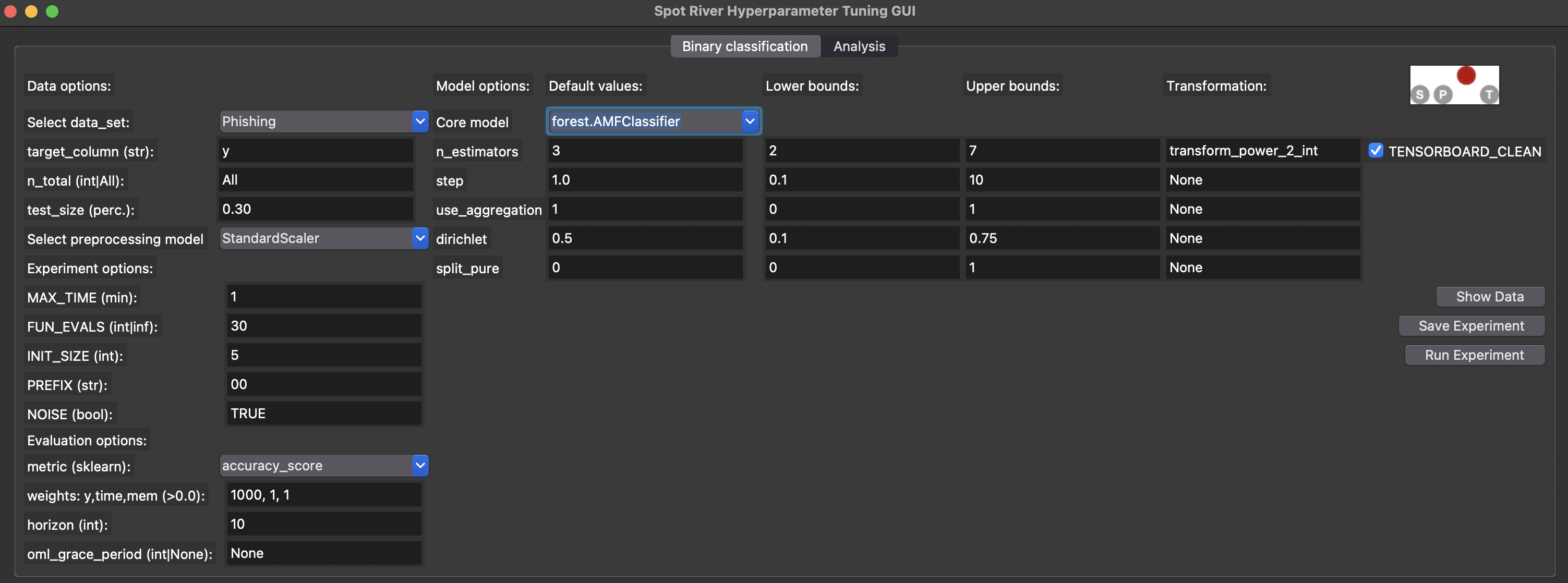
spotRiverGUI when forest.AMFClassifier is selected
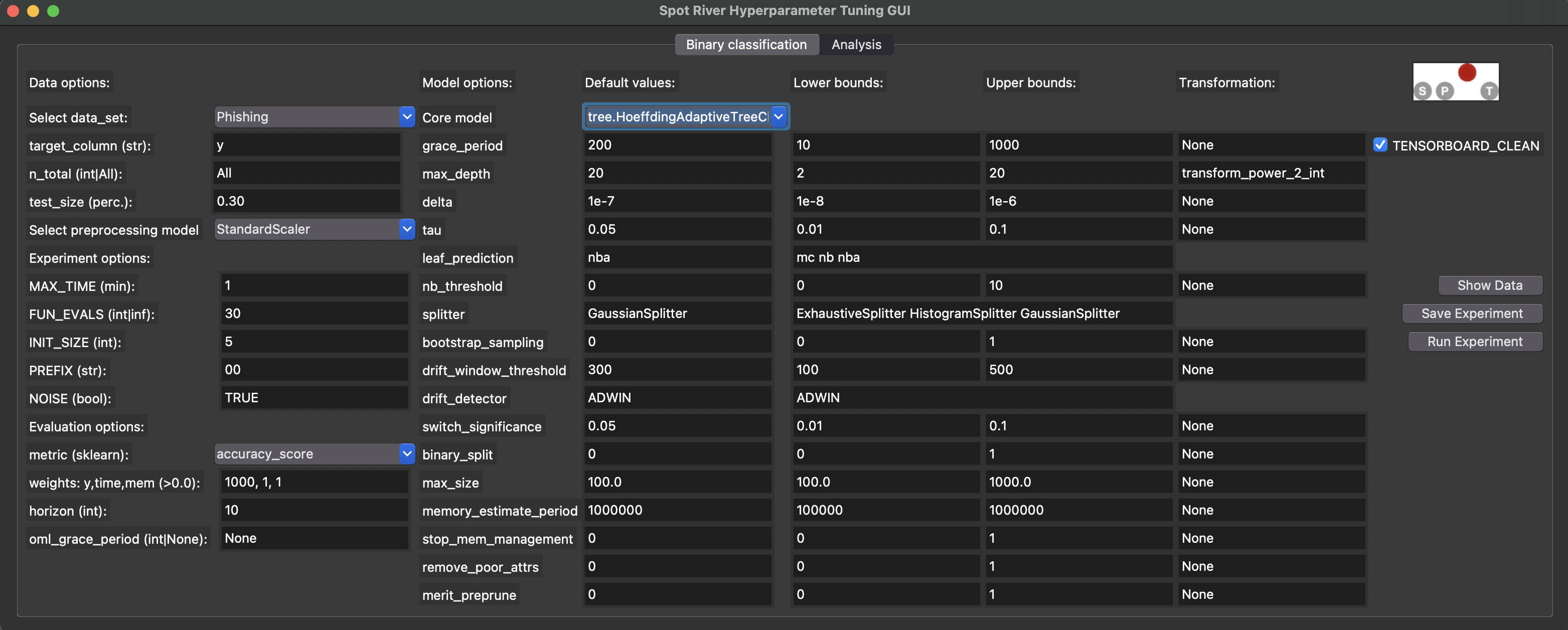
spotRiverGUI when tree.HoeffdingAdaptiveTreeClassifier is selected
Numerical and categorical hyperparameters are treated differently in the spotRiverGUI:
- The user can modify the lower and upper bounds for the numerical hyperparameters.
- There are no upper or lower bounds for categorical hyperparameters. Instead, hyperparameter values for the categorical hyperparameters are considered as sets of values, e.g., the set of
ExhaustiveSplitter,HistogramSplitter,GaussianSplitteris provided for thesplitterhyperparameter of thetree.HoeffdingAdaptiveTreeClassifiermodel as can be seen in Figure 19.3. The user can select the full set or any subset of the set of values for the categorical hyperparameters.
In addition to the lower and upper bounds (or the set of values for the categorical hyperparameters), the spotRiverGUI provides information about the Default values and the Transformation function. If the Transformation function is set to None, the values of the hyperparameters are passed to the spot tuner as they are. If the Transformation function is set to transform_power_2_int, the value \(x\) is transformed to \(2^x\) before it is passed to the spot tuner.
Modifications of the Default values and Transformation functions values in the spotRiverGUI have no effect on the hyperparameter tuning process. This is intensional. In future versions, the user will be able to add their own hyperparameter dictionaries to the spotRiverGUI, which allows the modification of Default values and Transformation functions values. Furthermore, the spotRiverGUI will support more online machine learning models in future versions.
19.4 Regression
Regression tasks will be supported soon. The same workflow as for the binary classification task will be used, i.e., the user can select the data set, the preprocessing model, the metric, and the online machine learning model.
19.5 Showing the Data
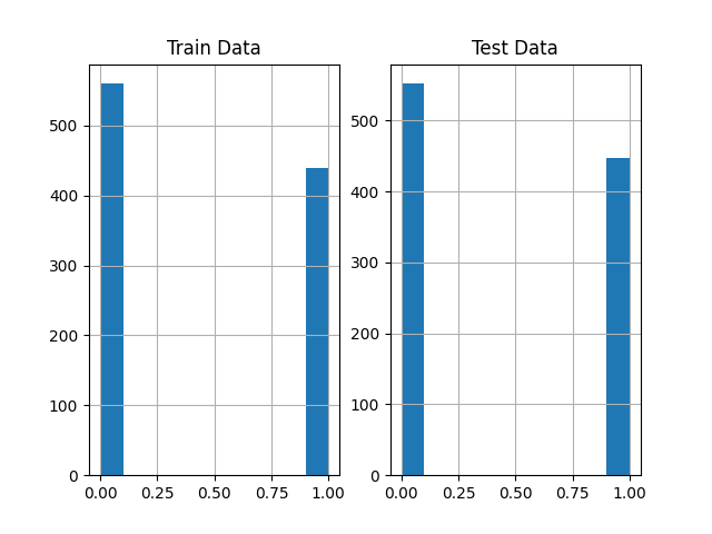
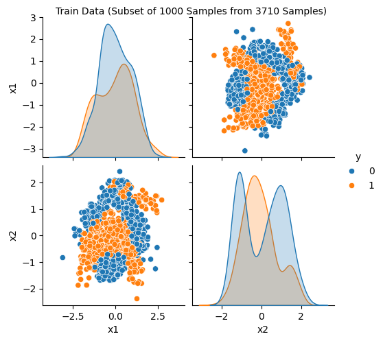
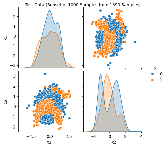
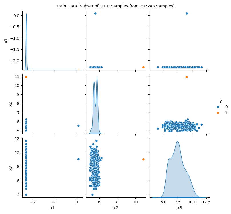
The spotRiverGUI provides the Show Data button, which opens a new window and shows information about the data set. The first figure (Figure 19.4) shows histograms of the target variables in the train and test data sets. The second figure (Figure 19.5) shows scatter plots of the features in the train data set. The third figure (Figure 19.6) shows the corresponding scatter plots of the features in the test data set.
spotRiverGUI when Bananas data is selected for the Show Data option
spotRiverGUI when Bananas data is selected for the Show Data option
spotRiverGUI when Bananas data is selected for the Show Data option
- Some data sets are quite large and the display of the data sets might take some time.
- Therefore, a random subset of 1000 instances of the data set is displayed if the data set is larger than 1000 instances.
Showing the data is important, especially for the new / unknown data sets as can be seen in Figure 19.7, Figure 19.8, and Figure 19.9: The target variable is highly biased. The user can check whether the data set is correctly formatted and whether the target variable is correctly specified.
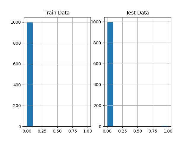
spotRiverGUI when HTTP data is selected for the Show Data option. The target variable is biased.
spotRiverGUI when HTTP data is selected for the Show Data option. A subset of 1000 randomly chosen data points is shown. Only a few positive events are in the data.
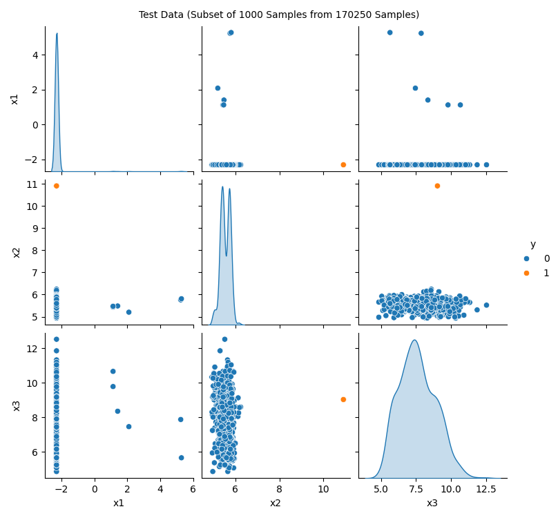
spotRiverGUI when HTTP data is selected for the Show Data option. The test data set shows the same structure as the train data set.
In addition to the histograms and scatter plots, the spotRiverGUI provides textual information about the data set in the console window. e.g., for the Bananas data set, the following information is shown:
Train data summary:
                 x1           x2            y
count  3710.000000  3710.000000  3710.000000
mean     -0.016243     0.002430     0.451482
std       0.995490     1.001150     0.497708
min      -3.089839    -2.385937     0.000000
25%      -0.764512    -0.914144     0.000000
50%      -0.027259    -0.033754     0.000000
75%       0.745066     0.836618     1.000000
max       2.754447     2.517112     1.000000

Test data summary:
                 x1           x2            y
count  1590.000000  1590.000000  1590.000000
mean      0.037900    -0.005670     0.440881
std       1.009744     0.997603     0.496649
min      -2.980834    -2.199138     0.000000
25%      -0.718710    -0.911151     0.000000
50%       0.034858    -0.046502     0.000000
75%       0.862049     0.806506     1.000000
max       2.813360     3.194302     1.000000
19.6 Saving and Loading
19.6.1 Saving the Experiment
If the experiment should not be started immediately, the user can save the experiment by clicking on the Save Experiment button. The spotRiverGUI will save the experiment as a pickle file. The file name is generated based on the PREFIX parameter. The pickle file contains a set of dictionaries, which are used to start the experiment.
spotRiverGUI shows a summary of the selected hyperparameters in the console window as can be seen in Table 19.1.
tree.HoeffdingAdaptiveTreeClassifier model.
| name | type | default | lower | upper | transform |
|---|---|---|---|---|---|
| grace_period | int | 200 | 10 | 1000 | None |
| max_depth | int | 20 | 2 | 20 | transform_power_2_int |
| delta | float | 1e-07 | 1e-08 | 1e-06 | None |
| tau | float | 0.05 | 0.01 | 0.1 | None |
| leaf_prediction | factor | nba | 0 | 2 | None |
| nb_threshold | int | 0 | 0 | 10 | None |
| splitter | factor | GaussianSplitter | 0 | 2 | None |
| bootstrap_sampling | factor | 0 | 0 | 1 | None |
| drift_window_threshold | int | 300 | 100 | 500 | None |
| drift_detector | factor | ADWIN | 0 | 0 | None |
| switch_significance | float | 0.05 | 0.01 | 0.1 | None |
| binary_split | factor | 0 | 0 | 1 | None |
| max_size | float | 100.0 | 100 | 1000 | None |
| memory_estimate_period | int | 1000000 | 100000 | 1e+06 | None |
| stop_mem_management | factor | 0 | 0 | 1 | None |
| remove_poor_attrs | factor | 0 | 0 | 1 | None |
| merit_preprune | factor | 0 | 0 | 1 | None |
19.6.2 Loading an Experiment
Future versions of the spotRiverGUI will support the loading of experiments from the GUI. Currently, the user can load the experiment by executing the command load_experiment, see https://sequential-parameter-optimization.github.io/spotPython/reference/spotPython/utils/file/#spotPython.utils.file.load_experiment.
19.7 Running a New Experiment
An experiment can be started by clicking on the Run Experiment button. The GUI calls run_spot_python_experiment from spotGUI.tuner.spotRun. Output will be shown in the console window from which the GUI was started.
19.7.1 Starting and Stopping Tensorboard
Tensorboard (Abadi et al. 2016) is automatically started when an experiment is started. The tensorboard process can be observed in a browser by opening the http://localhost:6006 page. Tensorboard provides a visual representation of the hyperparameter tuning process. Figure 19.10 and Figure 19.11 show the tensorboard page when the spotRiverGUI is performing the tuning process.
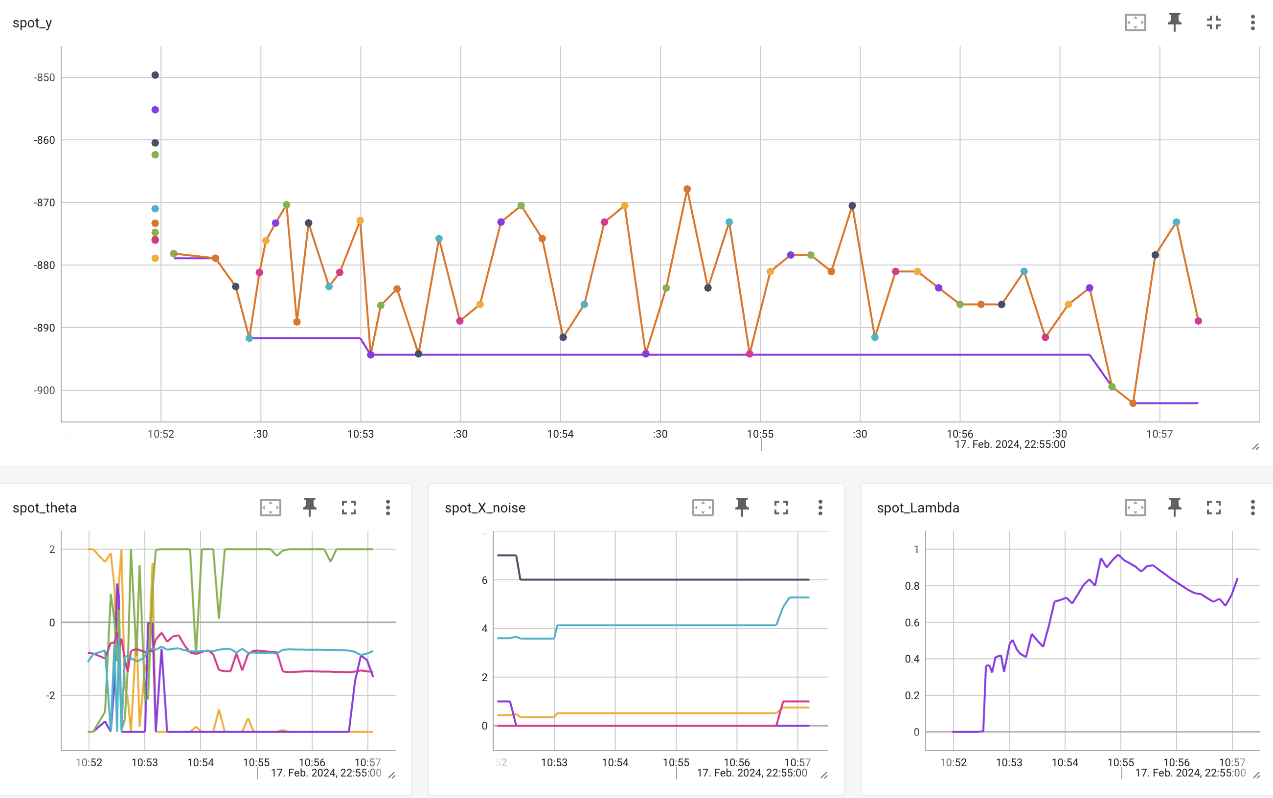
spotPython.utils.tensorboard provides the methods start_tensorboard and stop_tensorboard to start and stop tensorboard as a background process. After the experiment is finished, the tensorboard process is stopped automatically.
19.8 Performing the Analysis
If the hyperparameter tuning process is finished, the user can analyze the results by clicking on the Analysis button. The following options are available:
- Progress plot
- Compare tuned versus default hyperparameters
- Importance of hyperparameters
- Contour plot
- Parallel coordinates plot
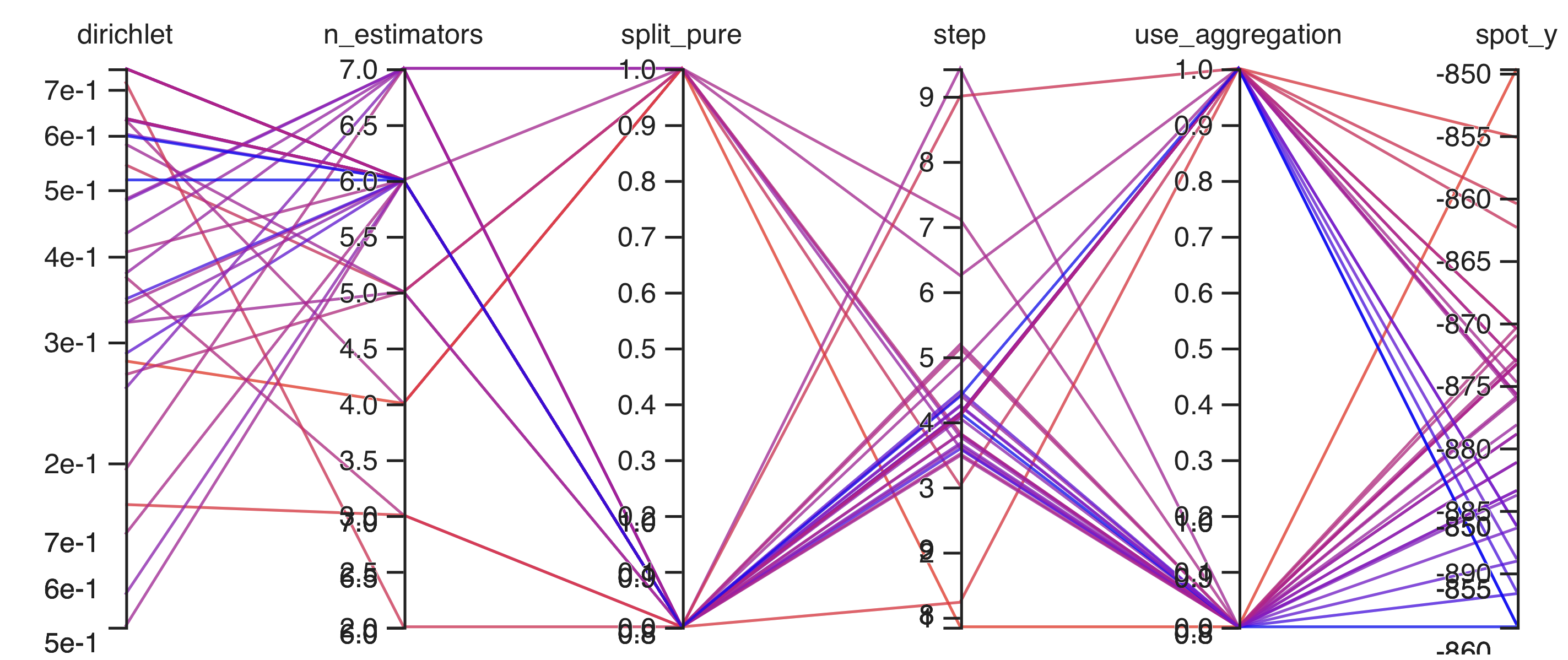
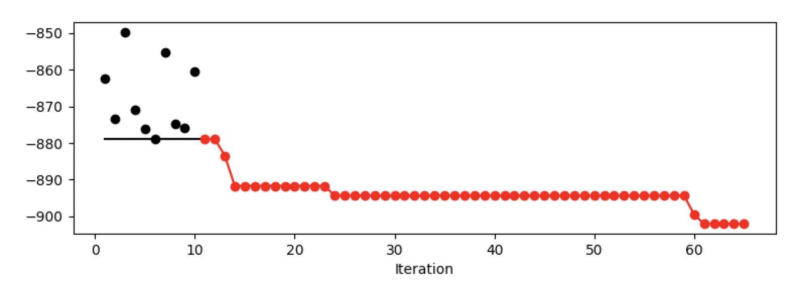
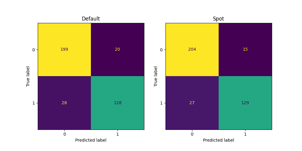
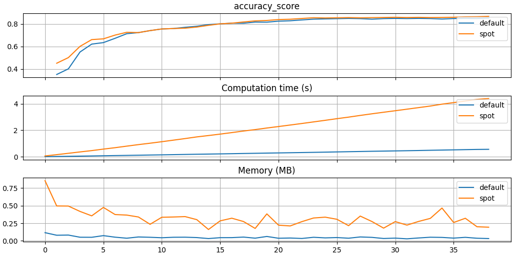
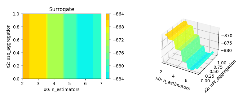
Figure 19.12 shows the progress plot of the hyperparameter tuning process. Black dots denote results from the initial design. Red dots illustrate the improvement found by the surrogate model based optimization. For binary classification tasks, the roc_auc_score can be used as the evaluation metric. The confusion matrix is shown in Figure 19.13. The default versus tuned hyperparameters are shown in Figure 19.14. The surrogate plot is shown in Figure 19.15, Figure 19.16, and Figure 19.17.
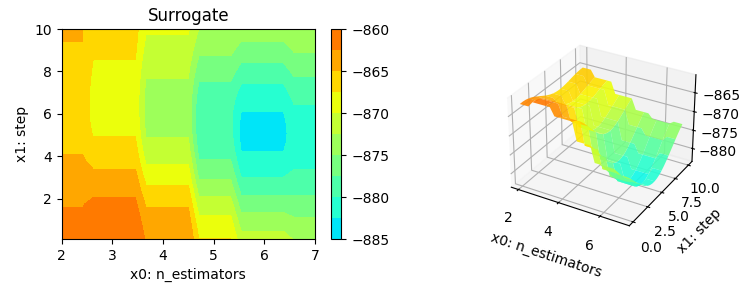
x0 and x1 plotted against each other.
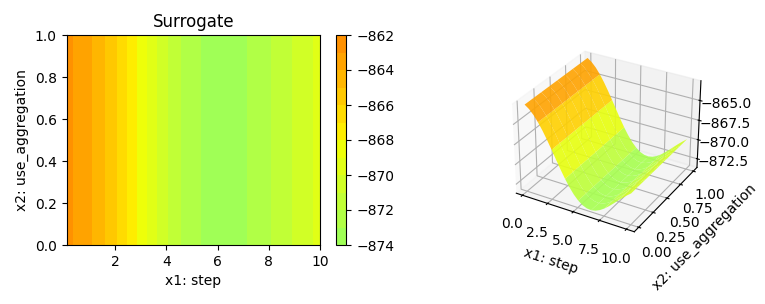
x1 and x2 plotted against each other.
x0 and x2 plotted against each other.
Furthermore, the tuned hyperparameters are shown in the console window. A typical output is shown below (modified due to formatting reasons):
|name    |type   |default |low | up |tuned |transf |importance|stars|
|--------|-------|--------|----|----|------|-------|----------|-----|
|n_estim |int    |    3.0 |2.0 |7.0 |  3.0 | pow_2 |      0.04|     |
|step    |float  |    1.0 |0.1 |10.0|  5.12| None  |      0.21| .   |
|use_agg |factor |    1.0 |0.0 |1.0 |  0.0 | None  |     10.17| *   |
|dirichl |float  |    0.5 |0.1 |0.75|  0.37| None  |     13.64| *   |
|split_p |factor |    0.0 |0.0 |1.0 |  0.0 | None  |    100.00| *** |
In addition to the tuned parameters that are shown in the column tuned, the columns importance and stars are shown. Both columns show the most important hyperparameters based on information from the surrogate model. The stars column shows the importance of the hyperparameters in a graphical way. It is important to note that the results are based on a demo of the hyperparameter tuning process. The plots are not based on a real hyperparameter tuning process. The reader is referred to Bartz-Beielstein (2024b) for further information about the analysis of the hyperparameter tuning process.
19.9 Summary and Outlook
The spotRiverGUI provides a graphical user interface for the spotRiver package. It releases the user from the burden of manually searching for the optimal hyperparameter setting. After copying a data set into the userData folder and starting spotRiverGUI, users can compare different OML algorithms from the powerful river package in a convenient way. Users can generate configurations on their local machines, which can be transferred to a remote machine for execution. Results from the remote machine can be copied back to the local machine for analysis.
- Very easy to use (only the data must be provided in the correct format).
- Reproducible results.
- State-of-the-art hyperparameter tuning methods.
- Powerful analysis tools, e.g., Bayesian optimization (Forrester, Sóbester, and Keane 2008; Gramacy 2020).
- Visual representation of the hyperparameter tuning process with tensorboard.
- Most advanced online machine learning models from the
riverpackage.
The river package (Montiel et al. 2021), which is very well documented, can be downloaded from https://riverml.xyz/latest/.
The spotRiverGUI is under active development and new features will be added soon. It can be downloaded from GitHub: https://github.com/sequential-parameter-optimization/spotGUI.
Interactive Jupyter Notebooks and further material about OML are provided in the GitHub repository https://github.com/sn-code-inside/online-machine-learning. This material is part of the supplementary material of the book “Online Machine Learning - A Practical Guide with Examples in Python”, see https://link.springer.com/book/9789819970063 and the forthcoming book “Online Machine Learning - Eine praxisorientierte Einführung”, see https://link.springer.com/book/9783658425043.