16  Surrogate Model Selection in SpotOptim

This section demonstrates how to select and configure different surrogate models in SpotOptim. We compare various surrogate options:

• Gaussian Process with different kernels (Matern, RBF, Rational Quadratic)
• SpotOptim Kriging model
• Random Forest regressor
• XGBoost regressor
• Support Vector Regression (SVR)
• Gradient Boosting regressor

All methods are evaluated on the Aircraft Wing Weight Example (AWWE) function. We visualize the fitted surrogates and compare optimization performance.

16.1 Introduction

SpotOptim supports any scikit-learn compatible regressor, allowing you to choose the surrogate that best fits your problem characteristics:

• Gaussian Processes: Provide uncertainty estimates, smooth interpolation, good for continuous functions. Support Expected Improvement (EI) acquisition.
• Kriging: Similar to GP but with customizable correlation functions. Supports EI acquisition.
• Random Forests: Robust to noise, handle discontinuities. Don’t provide uncertainty, so use acquisition='y' (greedy).
• XGBoost: Excellent for high-dimensional problems, fast training and prediction. Use acquisition='y'.
• SVR: Good for high-dimensional problems with smooth structure. Use acquisition='y'.
• Gradient Boosting: Strong performance on structured problems. Use acquisition='y'.

16.1.1 Acquisition Functions and Uncertainty

Models that provide uncertainty estimates (Gaussian Process, Kriging) work with all acquisition functions: ‘ei’ (Expected Improvement), ‘pi’ (Probability of Improvement), and ‘y’ (greedy).

Tree-based and other models (Random Forest, XGBoost, SVR, Gradient Boosting) don’t provide uncertainty estimates by default, so they should use acquisition='y' for greedy optimization. SpotOptim automatically handles this gracefully.

16.2 Setup and Imports

import numpy as np
import matplotlib.pyplot as plt
import pandas as pd
from spotoptim import SpotOptim
from spotoptim.surrogate import Kriging
import time
import warnings
warnings.filterwarnings('ignore')

# Scikit-learn models
from sklearn.gaussian_process import GaussianProcessRegressor
from sklearn.gaussian_process.kernels import (
    Matern, RBF, ConstantKernel, WhiteKernel, RationalQuadratic
)
from sklearn.ensemble import RandomForestRegressor, GradientBoostingRegressor
from sklearn.svm import SVR

• XGBoost (if available)

import os
os.environ["OMP_NUM_THREADS"] = "1"  # Prevent OpenMP conflict on macOS

try:
    import xgboost as xgb
    XGBOOST_AVAILABLE = True
except ImportError:
    XGBOOST_AVAILABLE = False
    print("XGBoost not available. Install with: pip install xgboost")

print("Libraries imported successfully!")

Libraries imported successfully!

16.3 The AWWE Objective Function

We use the Aircraft Wing Weight Example function, which models the weight of an unpainted light aircraft wing. The function accepts inputs in the unit cube \([0,1]^9\) and returns the wing weight in pounds.

from spotoptim.function.so import wingwt

# Problem setup
bounds = [(0, 1)] * 9
param_names = ['Sw', 'Wfw', 'A', 'L', 'q', 'l', 'Rtc', 'Nz', 'Wdg']
max_iter = 20
n_initial = 15
seed = 42

print(f"Problem dimension: {len(bounds)}")
print(f"Optimization budget: {max_iter} evaluations")

Problem dimension: 9
Optimization budget: 20 evaluations

16.4 1. Default Surrogate: Gaussian Process with Matern Kernel

SpotOptim’s default surrogate is a Gaussian Process with a Matern kernel (\(\nu\)=2.5), which provides twice-differentiable sample paths and good performance for most optimization problems.

start_time = time.time()

# Default GP (no surrogate specified)
optimizer_default = SpotOptim(
    fun=wingwt,
    bounds=bounds,
    max_iter=max_iter,
    n_initial=n_initial,
    var_name=param_names,
    acquisition='ei',
    seed=seed,
    verbose=False
)

result_default = optimizer_default.optimize()
time_default = time.time() - start_time

print(f"\nResults:")
print(f"  Best weight: {result_default.fun:.4f} lb")
print(f"  Function evaluations: {result_default.nfev}")
print(f"  Time: {time_default:.2f}s")
print(f"  Success: {result_default.success}")

# Store for comparison
results_comparison = [{
    'Surrogate': 'GP Matern nu=2.5 (Default)',
    'Best Weight': result_default.fun,
    'Evaluations': result_default.nfev,
    'Time (s)': time_default,
    'Success': result_default.success
}]

Results:
  Best weight: 119.8664 lb
  Function evaluations: 20
  Time: 1.65s
  Success: True

16.4.1 Visualization: Default Surrogate

# Plot convergence
optimizer_default.plot_progress(log_y=False, figsize=(10, 5))

# Plot most important hyperparameters
optimizer_default.plot_important_hyperparameter_contour(max_imp=3)
plt.suptitle('Default GP Matern nu=2.5: Most Important Parameters', y=1.02)
plt.show()

Plotting surrogate contours for top 3 most important parameters:
  Nz: importance = 22.46% (type: float)
  A: importance = 20.27% (type: float)
  Rtc: importance = 17.83% (type: float)

Generating 3 surrogate plots...
  Plotting Nz vs A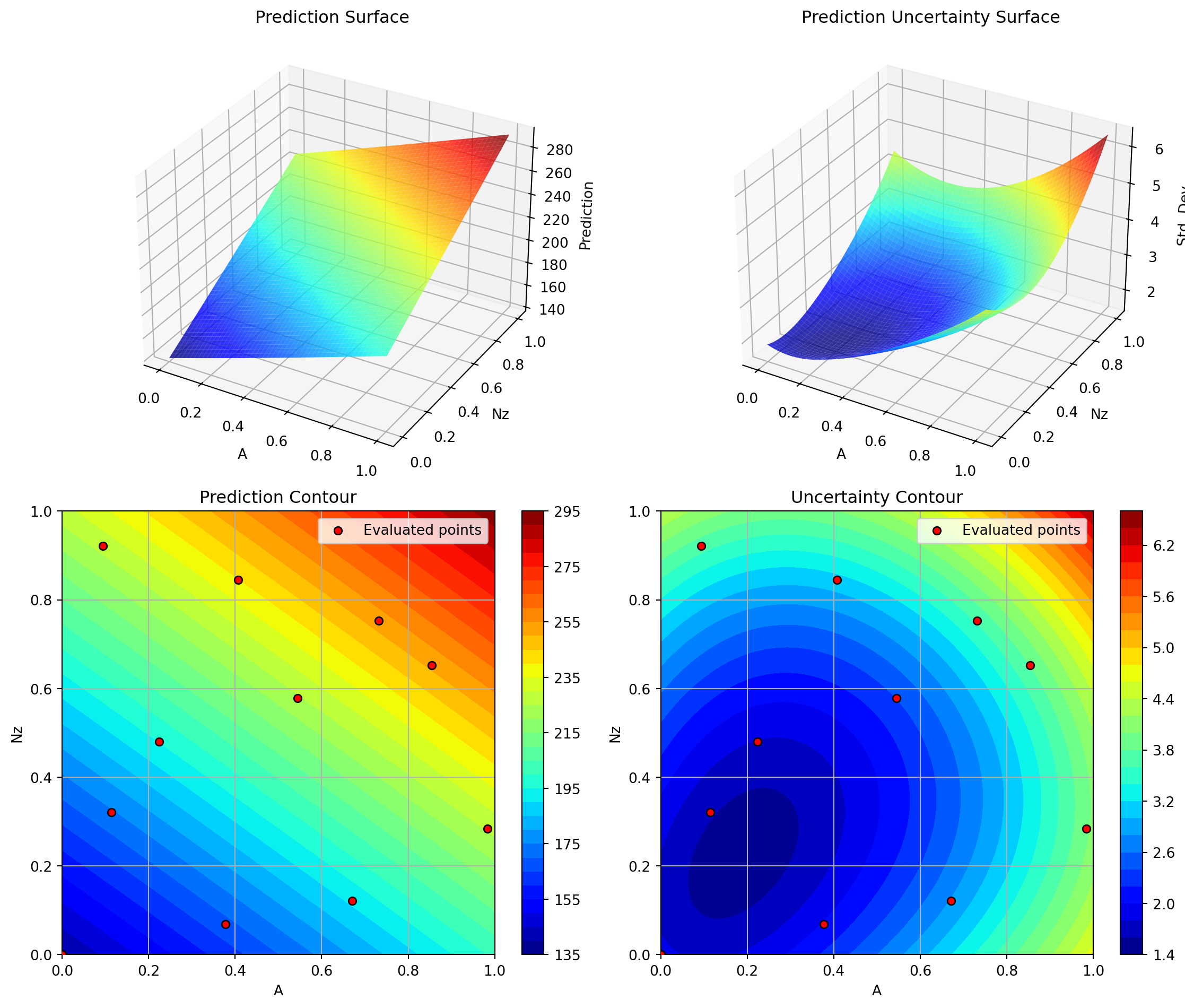

  Plotting Nz vs Rtc

  Plotting A vs Rtc

<Figure size 672x480 with 0 Axes>

16.5 2. Gaussian Process with RBF (Radial Basis Function) Kernel

The RBF kernel (also called squared exponential) produces infinitely differentiable sample paths, resulting in very smooth predictions.

start_time = time.time()

# Configure GP with RBF kernel
kernel_rbf = ConstantKernel(1.0, (1e-3, 1e3)) * RBF(
    length_scale=1.0, 
    length_scale_bounds=(1e-2, 1e2)
)

gp_rbf = GaussianProcessRegressor(
    kernel=kernel_rbf,
    n_restarts_optimizer=10,
    normalize_y=True,
    random_state=seed
)

optimizer_rbf = SpotOptim(
    fun=wingwt,
    bounds=bounds,
    surrogate=gp_rbf,
    max_iter=max_iter,
    n_initial=n_initial,
    var_name=param_names,
    acquisition='ei',
    seed=seed,
    verbose=False
)

result_rbf = optimizer_rbf.optimize()
time_rbf = time.time() - start_time

print(f"\nResults:")
print(f"  Best weight: {result_rbf.fun:.4f} lb")
print(f"  Function evaluations: {result_rbf.nfev}")
print(f"  Time: {time_rbf:.2f}s")
print(f"  Success: {result_rbf.success}")

results_comparison.append({
    'Surrogate': 'GP RBF',
    'Best Weight': result_rbf.fun,
    'Evaluations': result_rbf.nfev,
    'Time (s)': time_rbf,
    'Success': result_rbf.success
})

Results:
  Best weight: 120.1093 lb
  Function evaluations: 20
  Time: 0.47s
  Success: True

16.5.1 Visualization: RBF Kernel

optimizer_rbf.plot_progress(log_y=False, figsize=(10, 5))

optimizer_rbf.plot_important_hyperparameter_contour(max_imp=3)
plt.suptitle('GP RBF Kernel: Most Important Parameters', y=1.02)
plt.show()

Plotting surrogate contours for top 3 most important parameters:
  Nz: importance = 22.94% (type: float)
  A: importance = 20.71% (type: float)
  Rtc: importance = 18.21% (type: float)

Generating 3 surrogate plots...
  Plotting Nz vs A

  Plotting Nz vs Rtc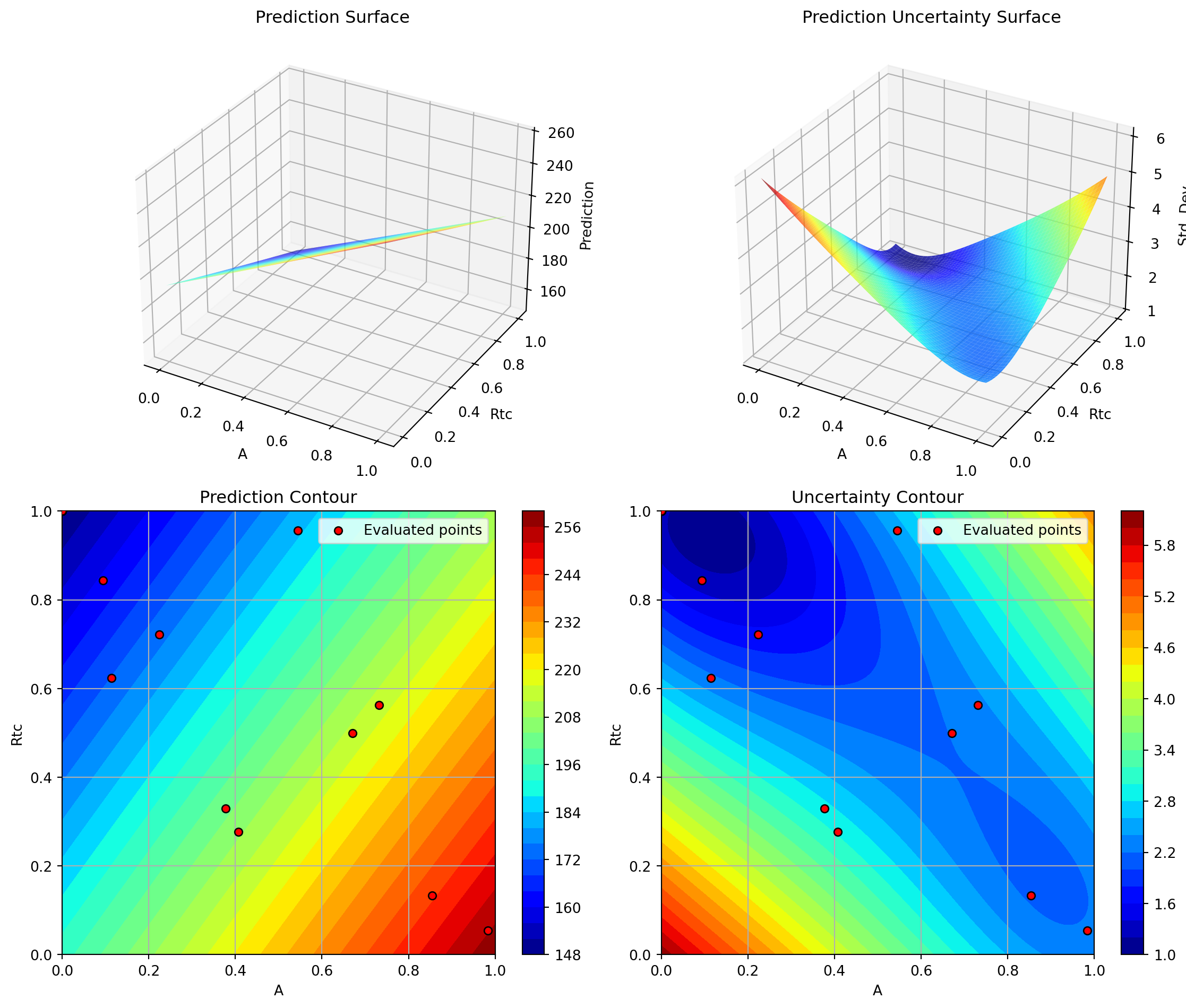

  Plotting A vs Rtc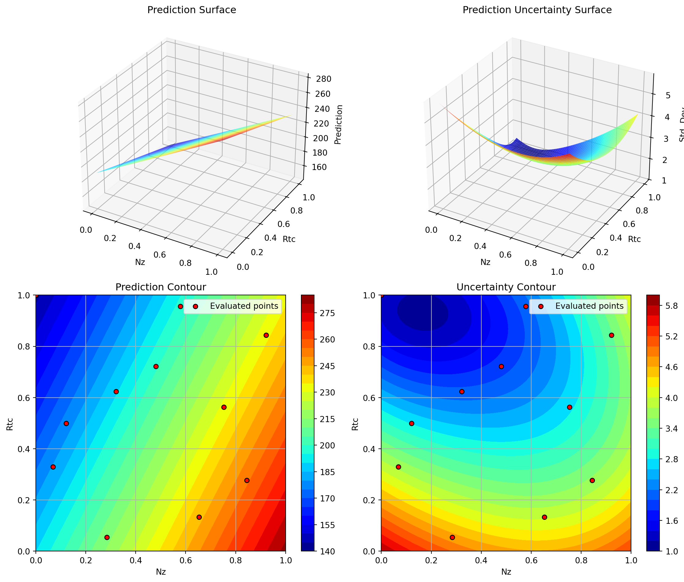

<Figure size 672x480 with 0 Axes>

16.6 3. Gaussian Process with Matern nu=1.5 Kernel

The Matern nu=1.5 kernel produces once-differentiable sample paths, allowing for more flexible (less smooth) fits than nu=2.5.

start_time = time.time()

# Configure GP with Matern nu=1.5
kernel_matern15 = ConstantKernel(1.0, (1e-3, 1e3)) * Matern(
    length_scale=1.0, 
    length_scale_bounds=(1e-2, 1e2),
    nu=1.5
)

gp_matern15 = GaussianProcessRegressor(
    kernel=kernel_matern15,
    n_restarts_optimizer=10,
    normalize_y=True,
    random_state=seed
)

optimizer_matern15 = SpotOptim(
    fun=wingwt,
    bounds=bounds,
    surrogate=gp_matern15,
    max_iter=max_iter,
    n_initial=n_initial,
    var_name=param_names,
    acquisition='ei',
    seed=seed,
    verbose=False
)

result_matern15 = optimizer_matern15.optimize()
time_matern15 = time.time() - start_time

print(f"\nResults:")
print(f"  Best weight: {result_matern15.fun:.4f} lb")
print(f"  Function evaluations: {result_matern15.nfev}")
print(f"  Time: {time_matern15:.2f}s")
print(f"  Success: {result_matern15.success}")

results_comparison.append({
    'Surrogate': 'GP Matern nu=1.5',
    'Best Weight': result_matern15.fun,
    'Evaluations': result_matern15.nfev,
    'Time (s)': time_matern15,
    'Success': result_matern15.success
})

Results:
  Best weight: 119.5465 lb
  Function evaluations: 20
  Time: 0.45s
  Success: True

16.6.1 Visualization: Matern nu=1.5 Kernel

optimizer_matern15.plot_progress(log_y=False, figsize=(10, 5))

optimizer_matern15.plot_important_hyperparameter_contour(max_imp=3)
plt.suptitle('GP Matern nu=1.5 Kernel: Most Important Parameters', y=1.02)
plt.show()

Plotting surrogate contours for top 3 most important parameters:
  Nz: importance = 22.42% (type: float)
  A: importance = 20.23% (type: float)
  Rtc: importance = 17.79% (type: float)

Generating 3 surrogate plots...
  Plotting Nz vs A

  Plotting Nz vs Rtc

  Plotting A vs Rtc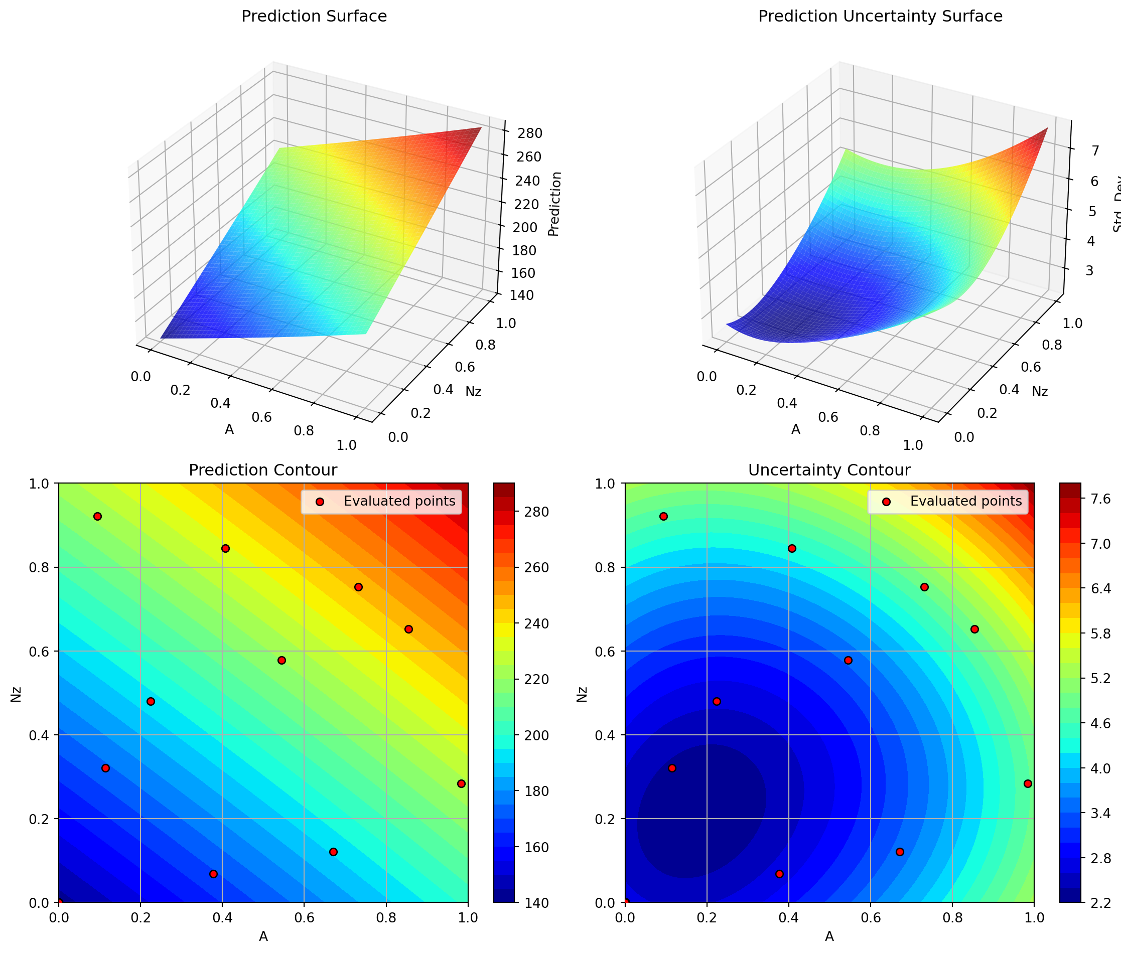

<Figure size 672x480 with 0 Axes>

16.7 4. Gaussian Process with Rational Quadratic Kernel

The Rational Quadratic kernel is a scale mixture of RBF kernels with different length scales, providing more flexibility than a single RBF.

start_time = time.time()

# Configure GP with Rational Quadratic kernel
kernel_rq = ConstantKernel(1.0, (1e-3, 1e3)) * RationalQuadratic(
    length_scale=1.0,
    alpha=1.0,
    length_scale_bounds=(1e-2, 1e2),
    alpha_bounds=(1e-2, 1e2)
)

gp_rq = GaussianProcessRegressor(
    kernel=kernel_rq,
    n_restarts_optimizer=10,
    normalize_y=True,
    random_state=seed
)

optimizer_rq = SpotOptim(
    fun=wingwt,
    bounds=bounds,
    surrogate=gp_rq,
    max_iter=max_iter,
    n_initial=n_initial,
    var_name=param_names,
    acquisition='ei',
    seed=seed,
    verbose=False
)

result_rq = optimizer_rq.optimize()
time_rq = time.time() - start_time

print(f"\nResults:")
print(f"  Best weight: {result_rq.fun:.4f} lb")
print(f"  Function evaluations: {result_rq.nfev}")
print(f"  Time: {time_rq:.2f}s")
print(f"  Success: {result_rq.success}")

results_comparison.append({
    'Surrogate': 'GP Rational Quadratic',
    'Best Weight': result_rq.fun,
    'Evaluations': result_rq.nfev,
    'Time (s)': time_rq,
    'Success': result_rq.success
})

Results:
  Best weight: 120.1073 lb
  Function evaluations: 20
  Time: 0.62s
  Success: True

16.7.1 Visualization: Rational Quadratic Kernel

optimizer_rq.plot_progress(log_y=False, figsize=(10, 5))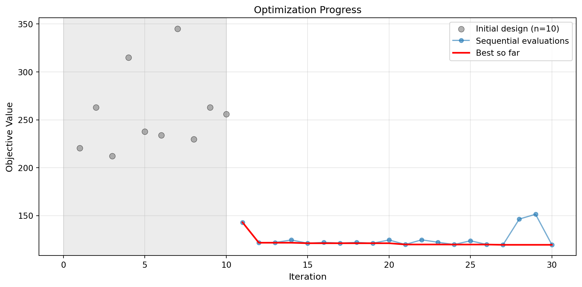

optimizer_rq.plot_important_hyperparameter_contour(max_imp=3)
plt.suptitle('GP Rational Quadratic Kernel: Most Important Parameters', y=1.02)
plt.show()

Plotting surrogate contours for top 3 most important parameters:
  Nz: importance = 22.88% (type: float)
  A: importance = 20.64% (type: float)
  Rtc: importance = 18.16% (type: float)

Generating 3 surrogate plots...
  Plotting Nz vs A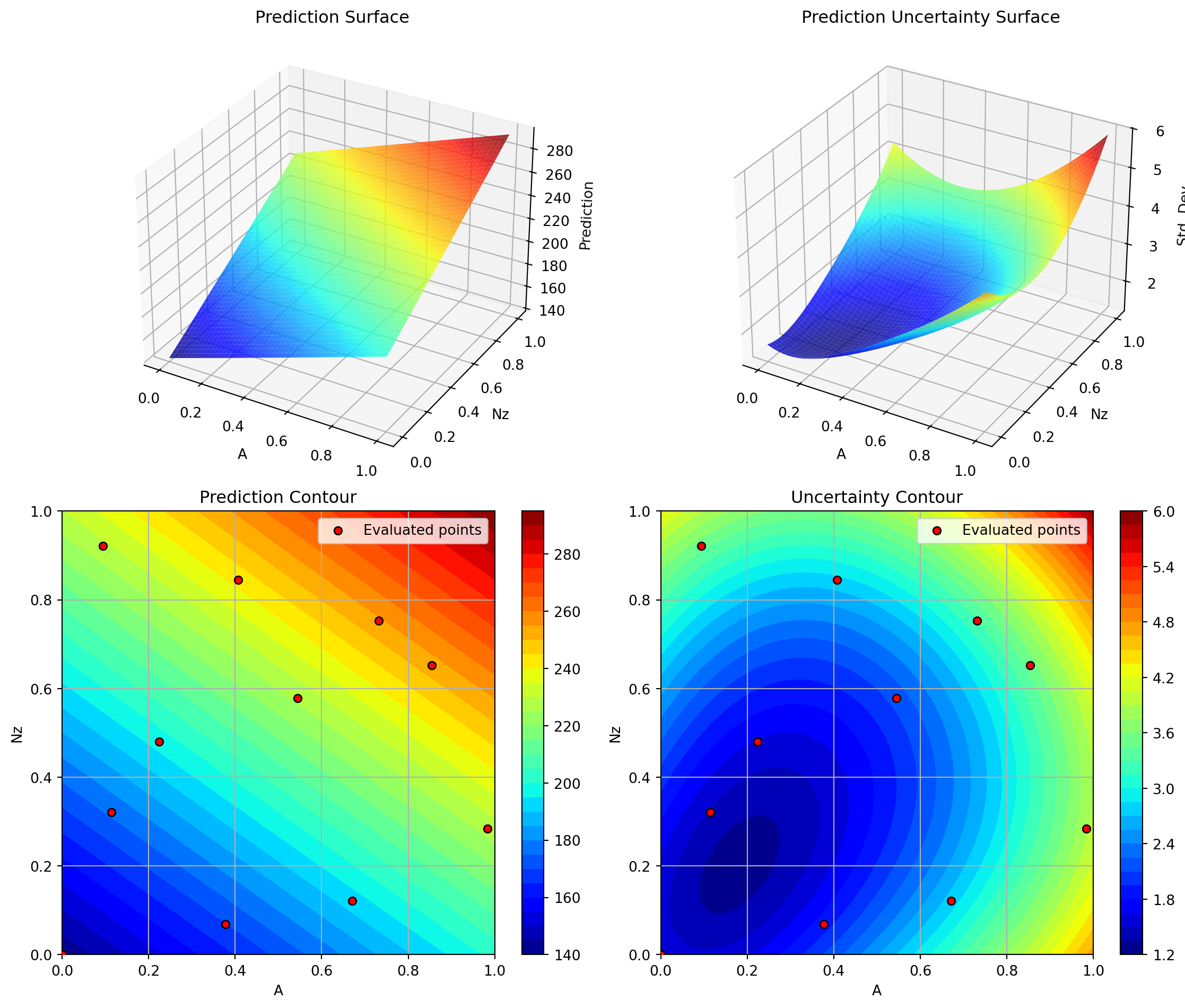

  Plotting Nz vs Rtc

  Plotting A vs Rtc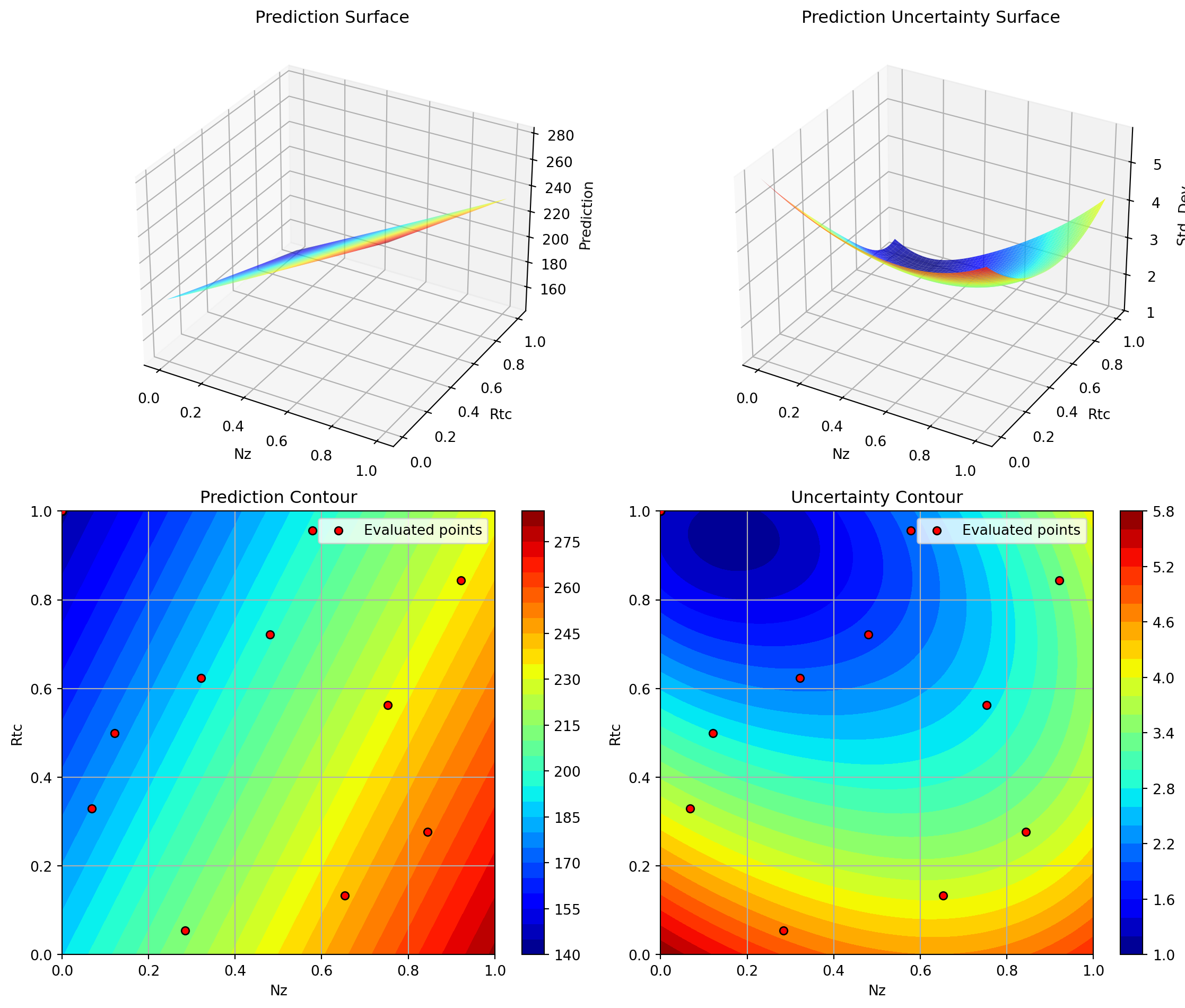

<Figure size 672x480 with 0 Axes>

16.8 5. SpotOptim Kriging Model

SpotOptim includes its own Kriging implementation optimized for sequential design. It uses Gaussian correlation function and optimizes hyperparameters via differential evolution.

start_time = time.time()

# Configure Kriging model
kriging_model = Kriging(
    noise=1e-10,          # Regularization parameter
    kernel='gauss',       # Gaussian/RBF kernel
    n_theta=None,         # Auto: use number of dimensions
    min_theta=-3.0,       # Min log10(theta) bound
    max_theta=2.0,        # Max log10(theta) bound
    seed=seed
)

optimizer_kriging = SpotOptim(
    fun=wingwt,
    bounds=bounds,
    surrogate=kriging_model,
    max_iter=max_iter,
    n_initial=n_initial,
    var_name=param_names,
    acquisition='ei',
    seed=seed,
    verbose=False
)

result_kriging = optimizer_kriging.optimize()
time_kriging = time.time() - start_time

print(f"\nResults:")
print(f"  Best weight: {result_kriging.fun:.4f} lb")
print(f"  Function evaluations: {result_kriging.nfev}")
print(f"  Time: {time_kriging:.2f}s")
print(f"  Success: {result_kriging.success}")

results_comparison.append({
    'Surrogate': 'SpotOptim Kriging',
    'Best Weight': result_kriging.fun,
    'Evaluations': result_kriging.nfev,
    'Time (s)': time_kriging,
    'Success': result_kriging.success
})

Results:
  Best weight: 121.2932 lb
  Function evaluations: 20
  Time: 8.08s
  Success: True

16.8.1 Visualization: Kriging Model

optimizer_kriging.plot_progress(log_y=False, figsize=(10, 5))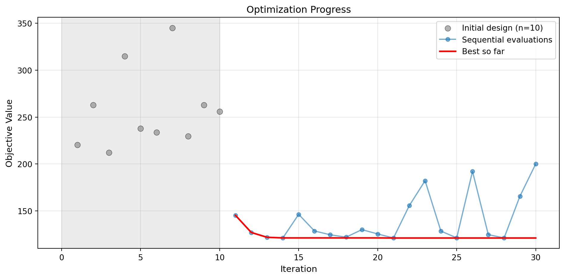

optimizer_kriging.plot_important_hyperparameter_contour(max_imp=3)
plt.suptitle('SpotOptim Kriging: Most Important Parameters', y=1.02)
plt.show()

Plotting surrogate contours for top 3 most important parameters:
  Nz: importance = 20.85% (type: float)
  A: importance = 18.80% (type: float)
  Rtc: importance = 16.51% (type: float)

Generating 3 surrogate plots...
  Plotting Nz vs A

  Plotting Nz vs Rtc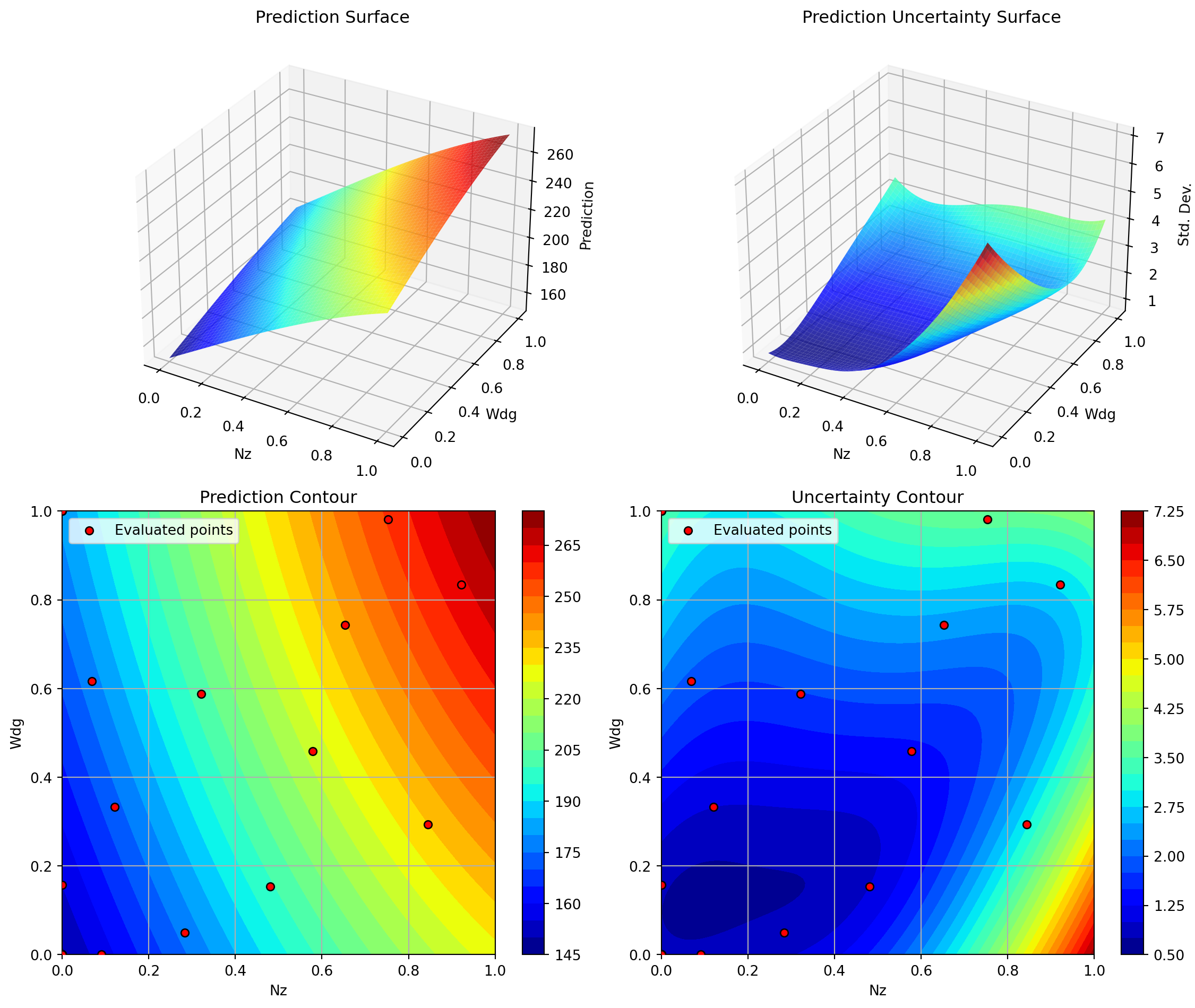

  Plotting A vs Rtc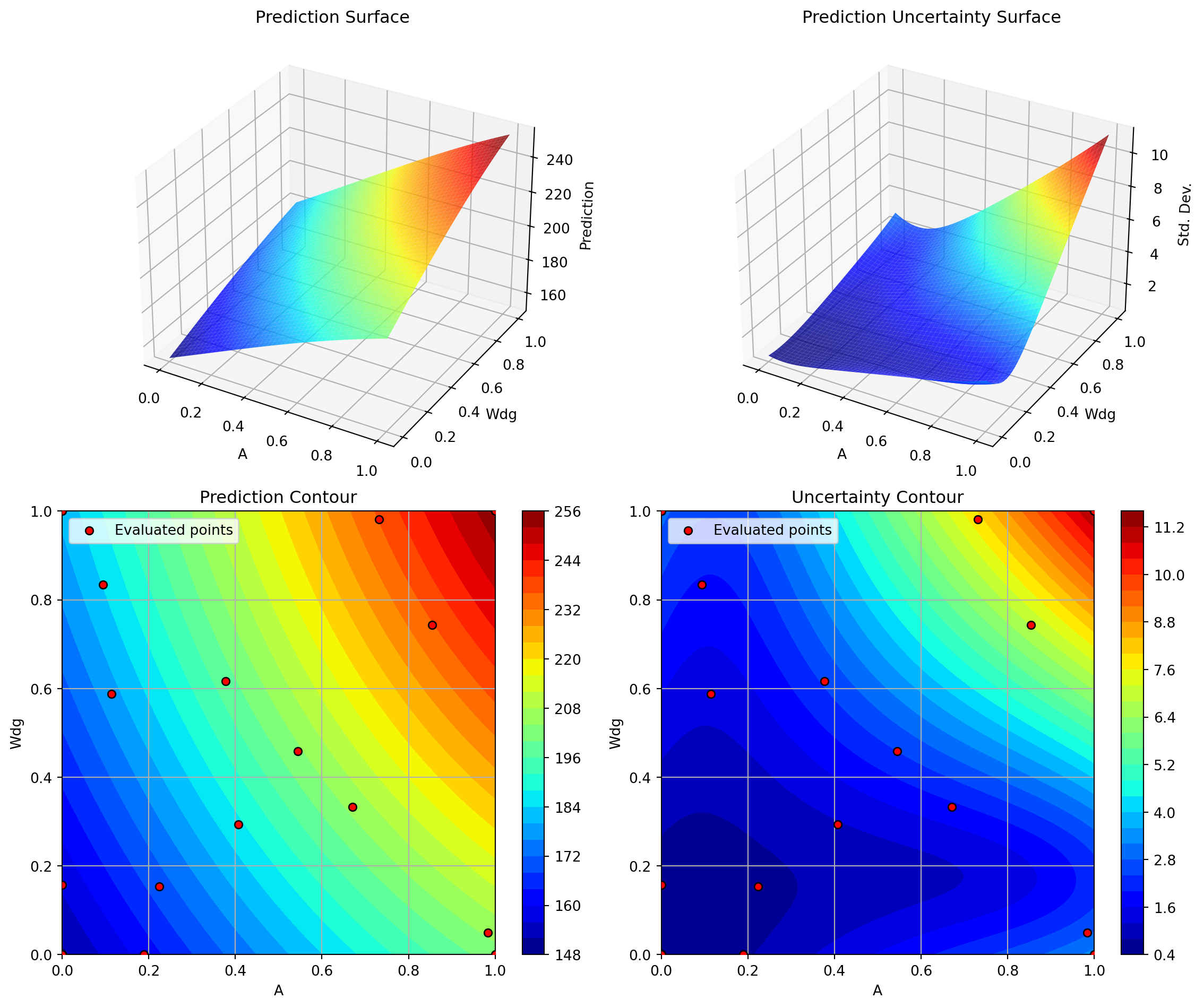

<Figure size 672x480 with 0 Axes>

16.9 6. Random Forest Regressor

Random Forests are ensemble methods that handle noise well and can model discontinuities. They don’t naturally provide uncertainty estimates, so the acquisition function uses predictions only.

start_time = time.time()

# Configure Random Forest
rf_model = RandomForestRegressor(
    n_estimators=100,
    max_depth=15,
    min_samples_split=2,
    min_samples_leaf=1,
    random_state=seed,
)

optimizer_rf = SpotOptim(
    fun=wingwt,
    bounds=bounds,
    surrogate=rf_model,
    max_iter=max_iter,
    n_initial=n_initial,
    var_name=param_names,
    acquisition='y',  # Use 'y' (greedy) since RF doesn't provide std
    seed=seed,
    verbose=False
)

result_rf = optimizer_rf.optimize()
time_rf = time.time() - start_time

print(f"\nResults:")
print(f"  Best weight: {result_rf.fun:.4f} lb")
print(f"  Function evaluations: {result_rf.nfev}")
print(f"  Time: {time_rf:.2f}s")
print(f"  Success: {result_rf.success}")
print(f"  Note: Using acquisition='y' (greedy) since RF doesn't provide uncertainty")

results_comparison.append({
    'Surrogate': 'Random Forest',
    'Best Weight': result_rf.fun,
    'Evaluations': result_rf.nfev,
    'Time (s)': time_rf,
    'Success': result_rf.success
})

Results:
  Best weight: 145.9792 lb
  Function evaluations: 20
  Time: 0.87s
  Success: True
  Note: Using acquisition='y' (greedy) since RF doesn't provide uncertainty

16.9.1 Visualization: Random Forest

optimizer_rf.plot_progress(log_y=False, figsize=(10, 5))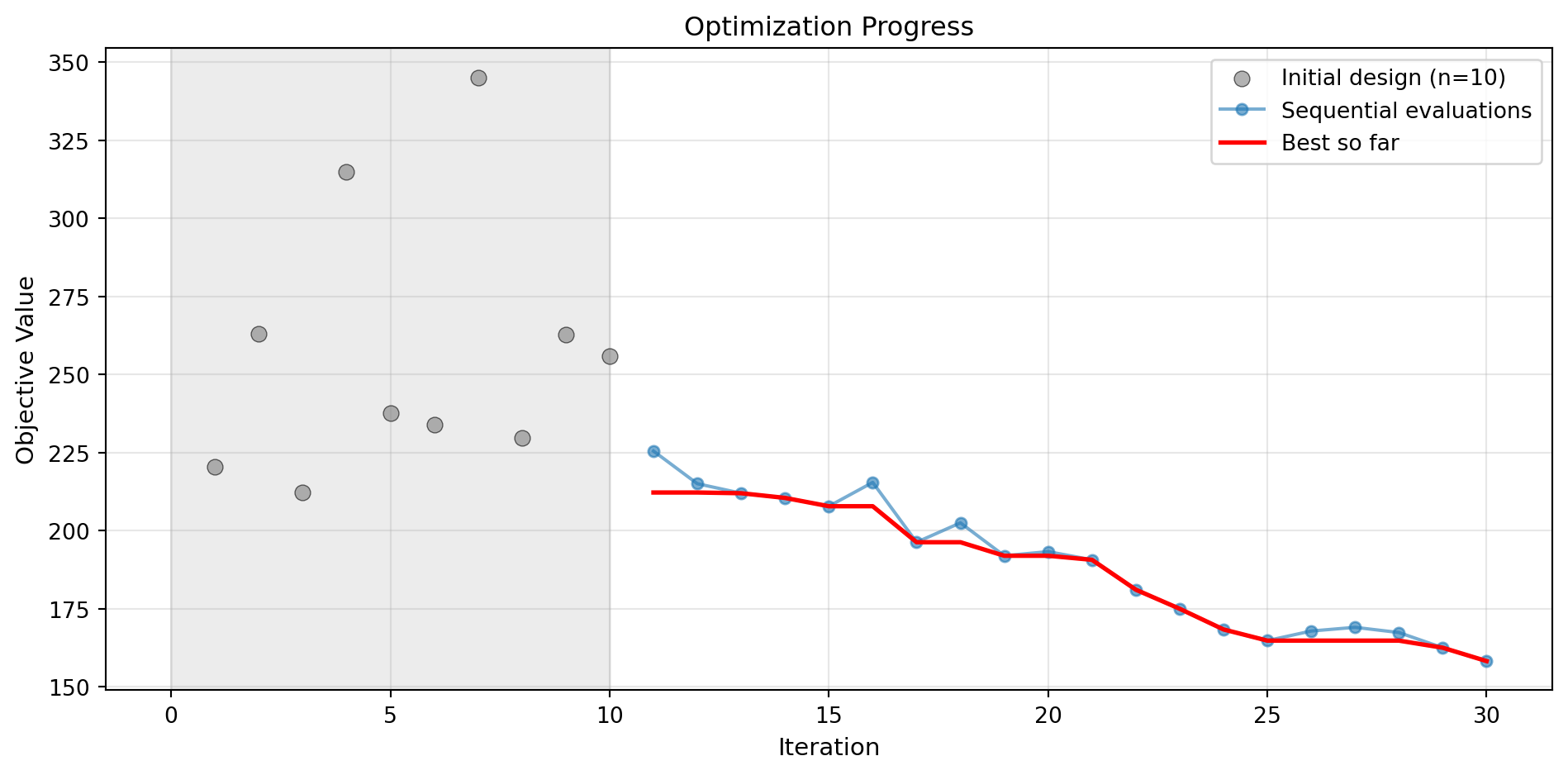

optimizer_rf.plot_important_hyperparameter_contour(max_imp=3)
plt.suptitle('Random Forest: Most Important Parameters', y=1.02)
plt.show()

Plotting surrogate contours for top 3 most important parameters:
  Nz: importance = 21.66% (type: float)
  A: importance = 19.61% (type: float)
  Rtc: importance = 15.41% (type: float)

Generating 3 surrogate plots...
  Plotting Nz vs A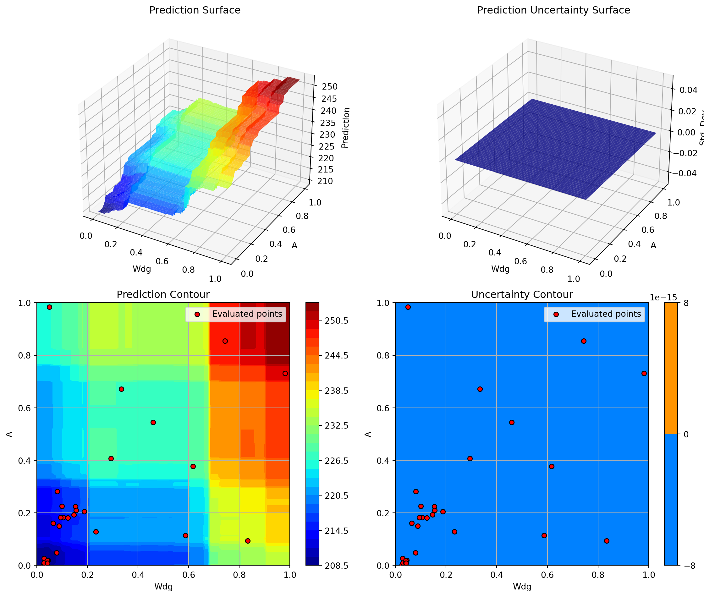

  Plotting Nz vs Rtc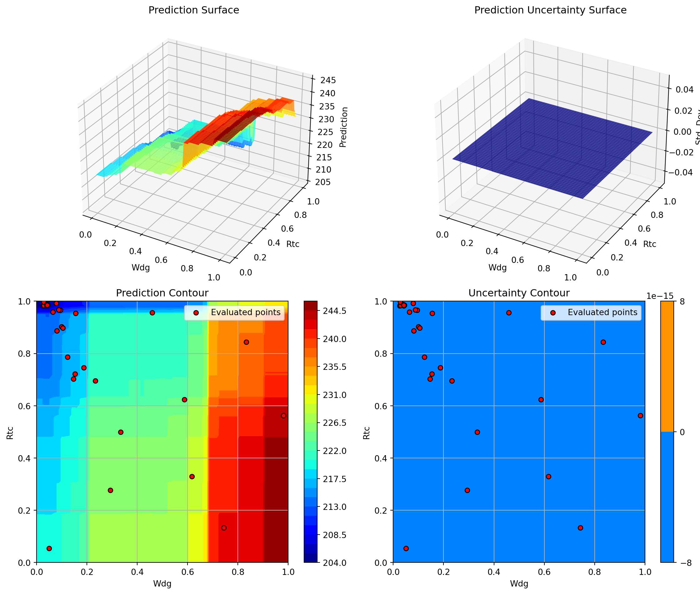

  Plotting A vs Rtc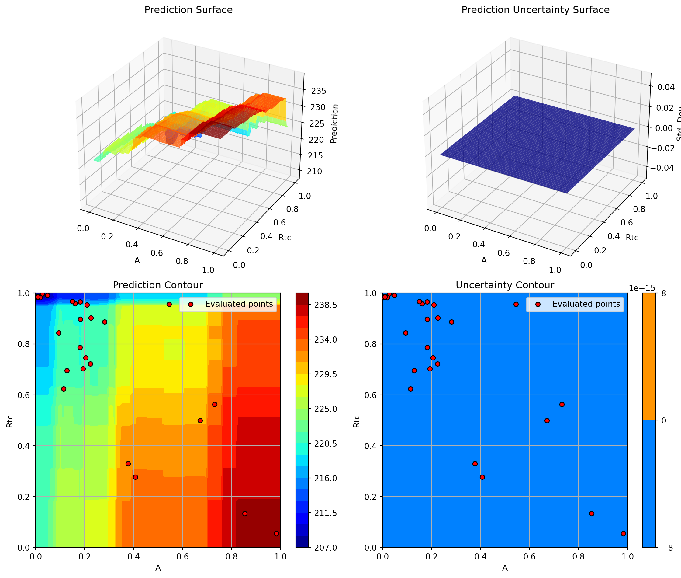

<Figure size 672x480 with 0 Axes>

16.10 7. XGBoost Regressor

XGBoost is a gradient boosting implementation known for excellent performance on structured data and fast training/prediction times.

if XGBOOST_AVAILABLE:
    start_time = time.time()
    
    # Configure XGBoost
    xgb_model = xgb.XGBRegressor(
        n_estimators=100,
        max_depth=6,
        learning_rate=0.1,
        subsample=0.8,
        colsample_bytree=0.8,
        random_state=seed,
        nthread=1,
        verbosity=0,
    )
    
    optimizer_xgb = SpotOptim(
        fun=wingwt,
        bounds=bounds,
        surrogate=xgb_model,
        max_iter=max_iter,
        n_initial=n_initial,
        var_name=param_names,
        acquisition='y',  # Use 'y' (greedy) since XGBoost doesn't provide std
        seed=seed,
        verbose=False
    )
    
    result_xgb = optimizer_xgb.optimize()
    time_xgb = time.time() - start_time
    
    print(f"\nResults:")
    print(f"  Best weight: {result_xgb.fun:.4f} lb")
    print(f"  Function evaluations: {result_xgb.nfev}")
    print(f"  Time: {time_xgb:.2f}s")
    print(f"  Success: {result_xgb.success}")
    print(f"  Note: Using acquisition='y' (greedy) since XGBoost doesn't provide uncertainty")
    
    results_comparison.append({
        'Surrogate': 'XGBoost',
        'Best Weight': result_xgb.fun,
        'Evaluations': result_xgb.nfev,
        'Time (s)': time_xgb,
        'Success': result_xgb.success
    })
    
    # Visualization
    optimizer_xgb.plot_progress(log_y=False, figsize=(10, 5))
    plt.title('XGBoost: Convergence')
    plt.show()
    
    optimizer_xgb.plot_important_hyperparameter_contour(max_imp=3)
    plt.suptitle('XGBoost: Most Important Parameters', y=1.02)
    plt.show()
else:
    print("=" * 80)
    print("7. XGBoost Regressor - SKIPPED (not installed)")
    print("=" * 80)
    print("Install XGBoost with: pip install xgboost")

Results:
  Best weight: 165.3064 lb
  Function evaluations: 20
  Time: 0.10s
  Success: True
  Note: Using acquisition='y' (greedy) since XGBoost doesn't provide uncertainty

Plotting surrogate contours for top 3 most important parameters:
  Nz: importance = 20.61% (type: float)
  A: importance = 18.24% (type: float)
  Rtc: importance = 14.07% (type: float)

Generating 3 surrogate plots...
  Plotting Nz vs A

  Plotting Nz vs Rtc

  Plotting A vs Rtc

<Figure size 672x480 with 0 Axes>

16.11 8. Support Vector Regression (SVR)

SVR with RBF kernel can model complex non-linear relationships. It’s particularly good for high-dimensional problems with smooth structure.

start_time = time.time()

# Configure SVR
svr_model = SVR(
    kernel='rbf',
    C=100.0,
    epsilon=0.1,
    gamma='scale'
)

optimizer_svr = SpotOptim(
    fun=wingwt,
    bounds=bounds,
    surrogate=svr_model,
    max_iter=max_iter,
    n_initial=n_initial,
    var_name=param_names,
    acquisition='y',  # Use 'y' (greedy) since SVR doesn't provide std by default
    seed=seed,
    verbose=False
)

result_svr = optimizer_svr.optimize()
time_svr = time.time() - start_time

print(f"\nResults:")
print(f"  Best weight: {result_svr.fun:.4f} lb")
print(f"  Function evaluations: {result_svr.nfev}")
print(f"  Time: {time_svr:.2f}s")
print(f"  Success: {result_svr.success}")

results_comparison.append({
    'Surrogate': 'SVR (RBF)',
    'Best Weight': result_svr.fun,
    'Evaluations': result_svr.nfev,
    'Time (s)': time_svr,
    'Success': result_svr.success
})

Results:
  Best weight: 156.7071 lb
  Function evaluations: 20
  Time: 0.07s
  Success: True

16.11.1 Visualization: SVR

optimizer_svr.plot_progress(log_y=False, figsize=(10, 5))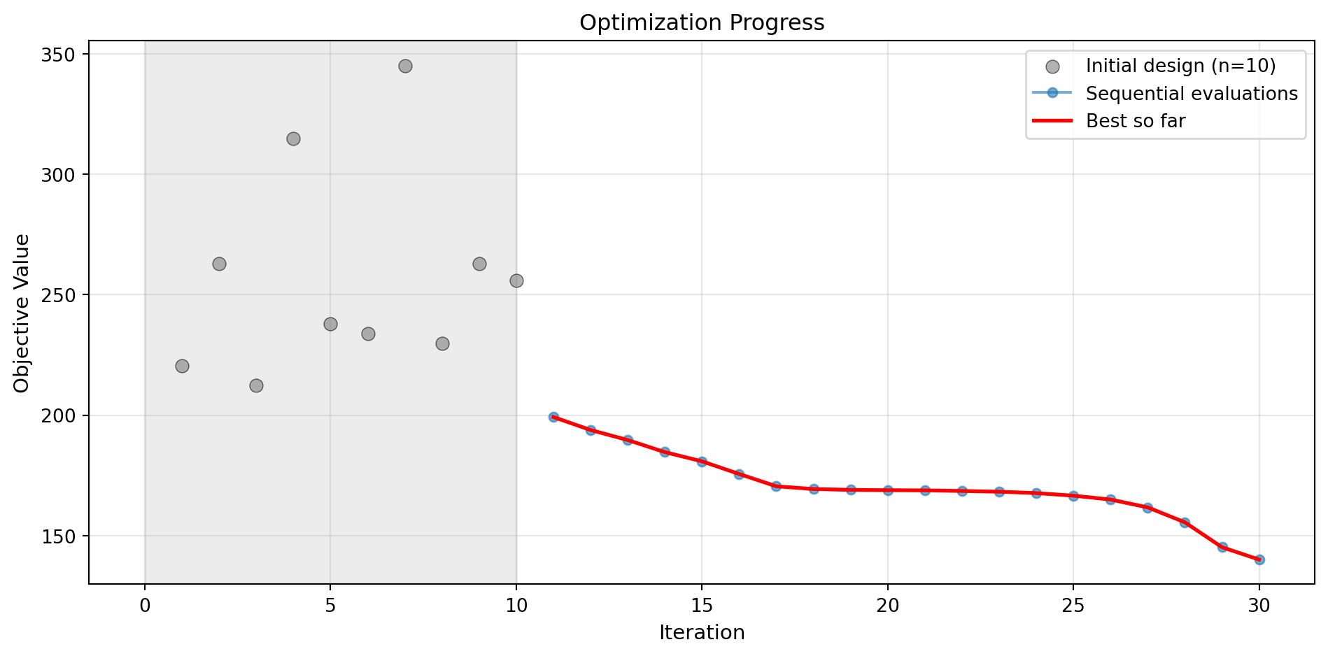

optimizer_svr.plot_important_hyperparameter_contour(max_imp=3)
plt.suptitle('Support Vector Regression: Most Important Parameters', y=1.02)
plt.show()

Plotting surrogate contours for top 3 most important parameters:
  Nz: importance = 25.67% (type: float)
  A: importance = 22.43% (type: float)
  Rtc: importance = 16.38% (type: float)

Generating 3 surrogate plots...
  Plotting Nz vs A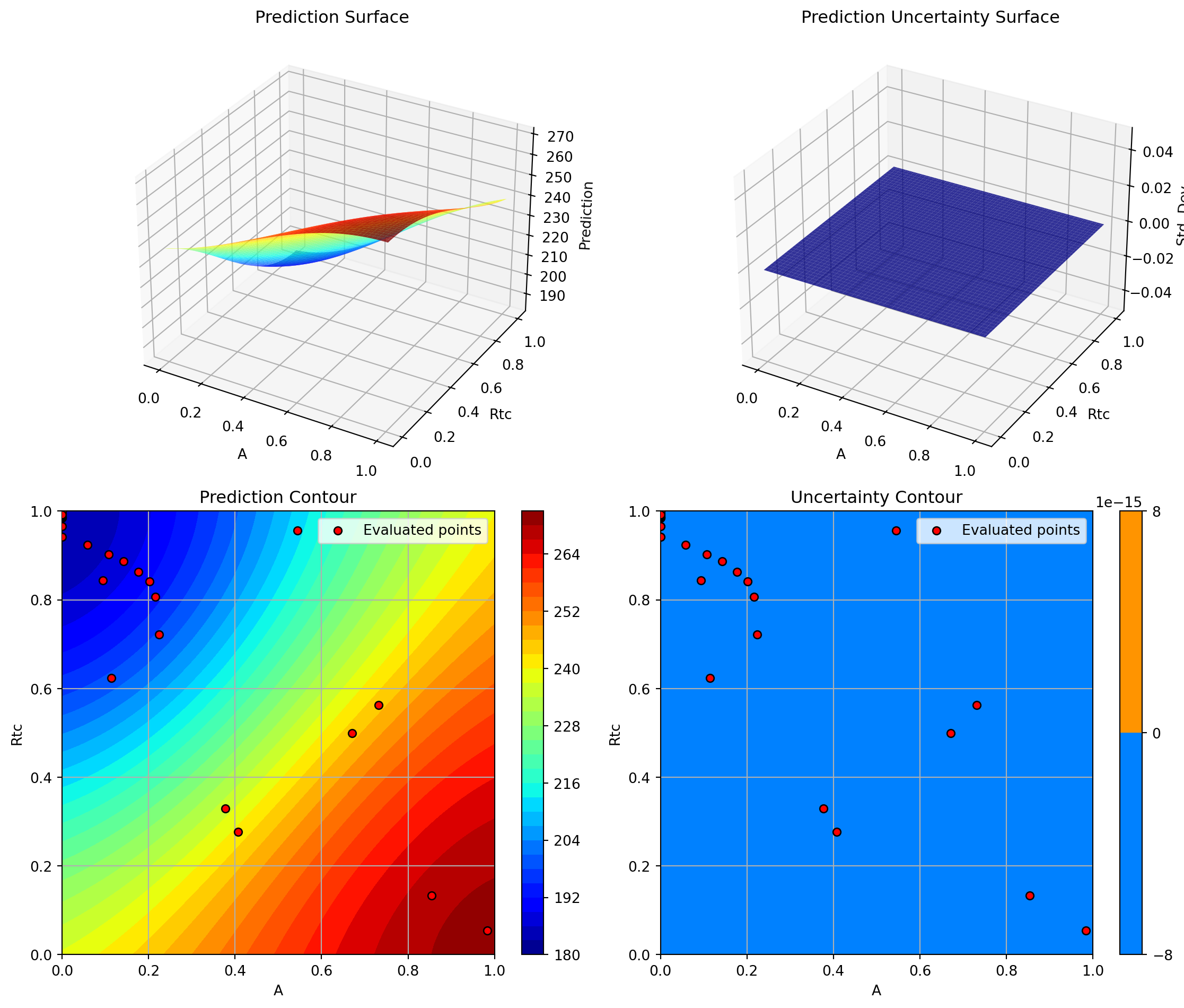

  Plotting Nz vs Rtc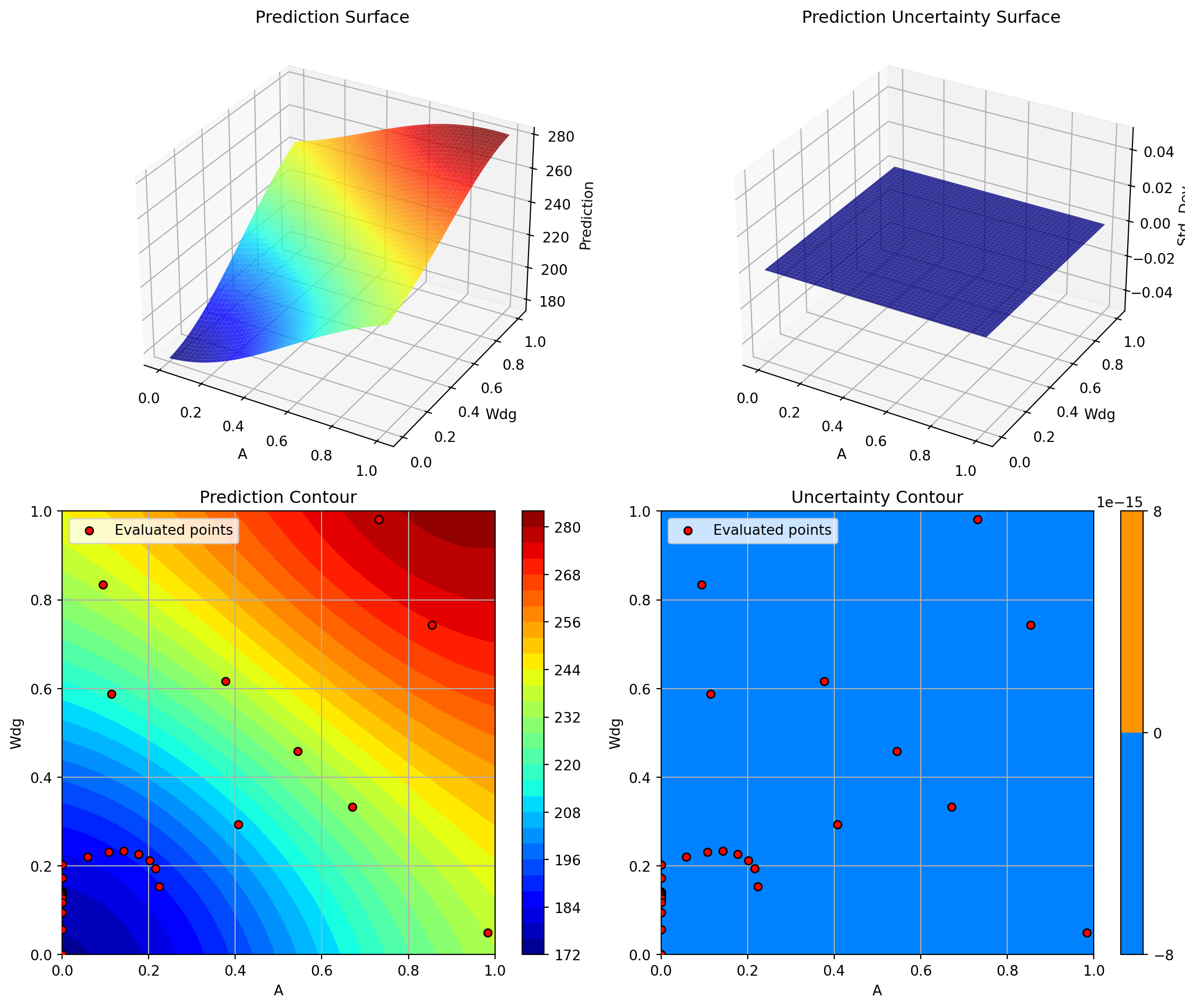

  Plotting A vs Rtc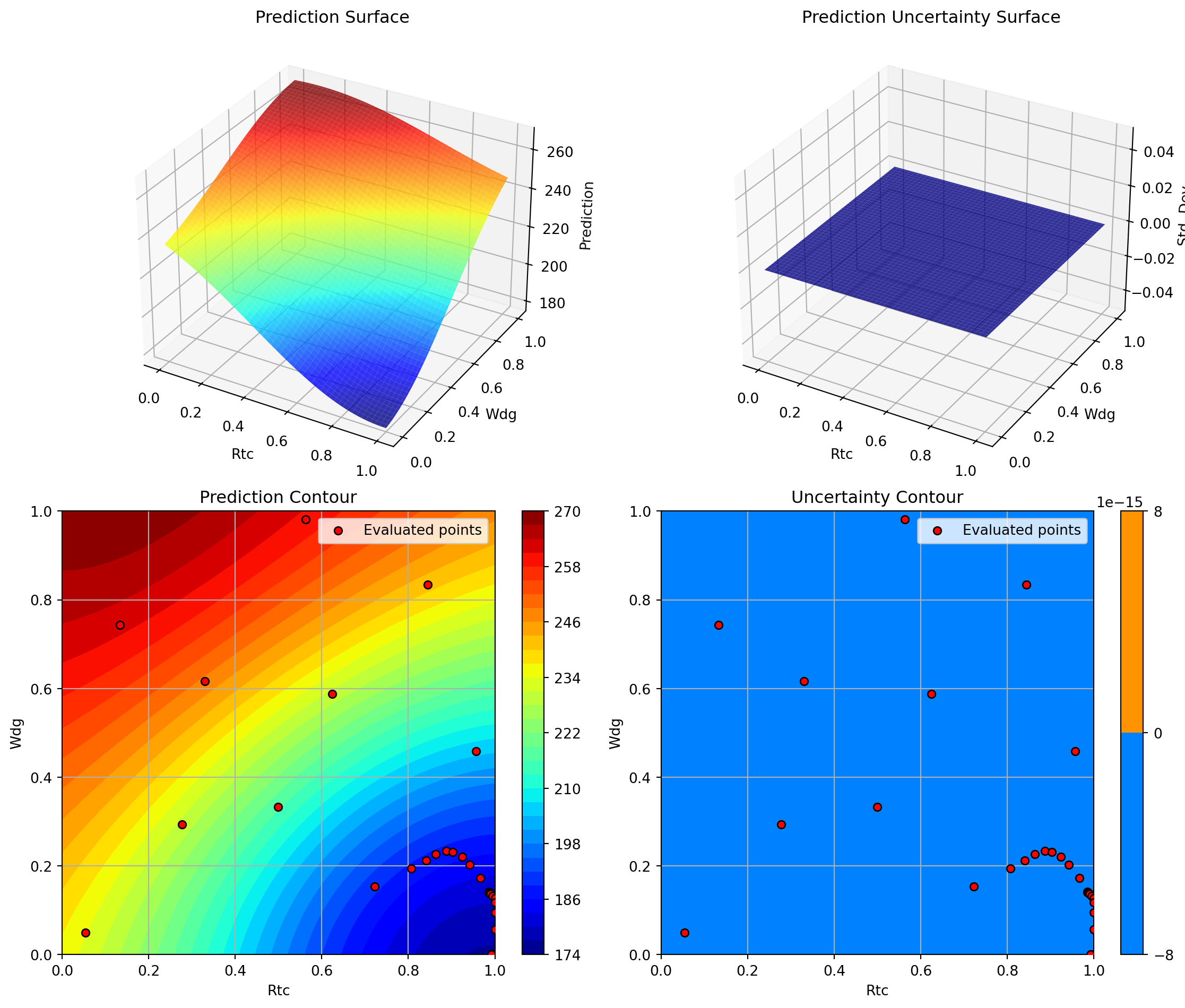

<Figure size 672x480 with 0 Axes>

16.12 9. Gradient Boosting Regressor

Gradient Boosting from scikit-learn is another ensemble method that builds trees sequentially, with each tree correcting errors of the previous ones.

start_time = time.time()

# Configure Gradient Boosting
gb_model = GradientBoostingRegressor(
    n_estimators=100,
    max_depth=5,
    learning_rate=0.1,
    subsample=0.8,
    random_state=seed
)

optimizer_gb = SpotOptim(
    fun=wingwt,
    bounds=bounds,
    surrogate=gb_model,
    max_iter=max_iter,
    n_initial=n_initial,
    var_name=param_names,
    acquisition='y',  # Use 'y' (greedy) since GB doesn't provide std
    seed=seed,
    verbose=False
)

result_gb = optimizer_gb.optimize()
time_gb = time.time() - start_time

print(f"\nResults:")
print(f"  Best weight: {result_gb.fun:.4f} lb")
print(f"  Function evaluations: {result_gb.nfev}")
print(f"  Time: {time_gb:.2f}s")
print(f"  Success: {result_gb.success}")

results_comparison.append({
    'Surrogate': 'Gradient Boosting',
    'Best Weight': result_gb.fun,
    'Evaluations': result_gb.nfev,
    'Time (s)': time_gb,
    'Success': result_gb.success
})

Results:
  Best weight: 134.5150 lb
  Function evaluations: 20
  Time: 0.18s
  Success: True

16.12.1 Visualization: Gradient Boosting

optimizer_gb.plot_progress(log_y=False, figsize=(10, 5))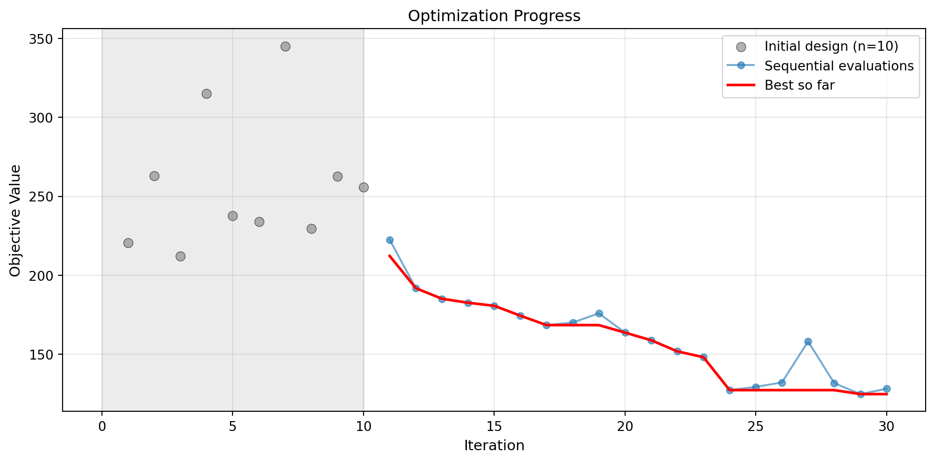

optimizer_gb.plot_important_hyperparameter_contour(max_imp=3)
plt.suptitle('Gradient Boosting: Most Important Parameters', y=1.02)
plt.show()

Plotting surrogate contours for top 3 most important parameters:
  Nz: importance = 19.99% (type: float)
  A: importance = 17.64% (type: float)
  Rtc: importance = 14.62% (type: float)

Generating 3 surrogate plots...
  Plotting Nz vs A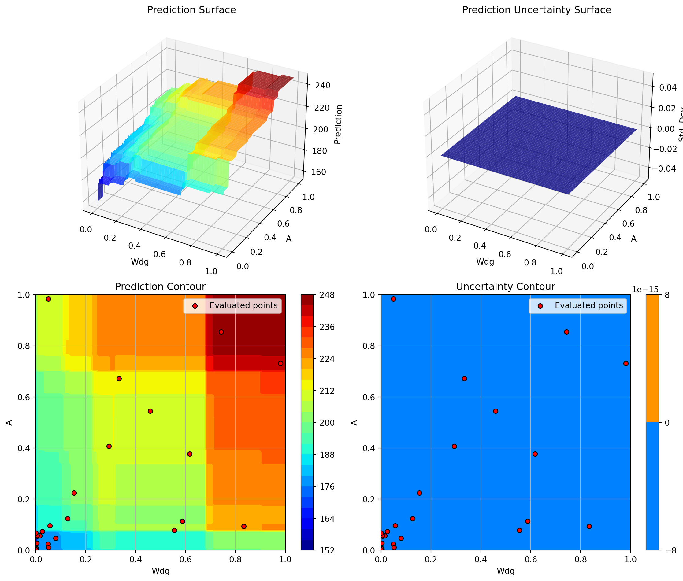

  Plotting Nz vs Rtc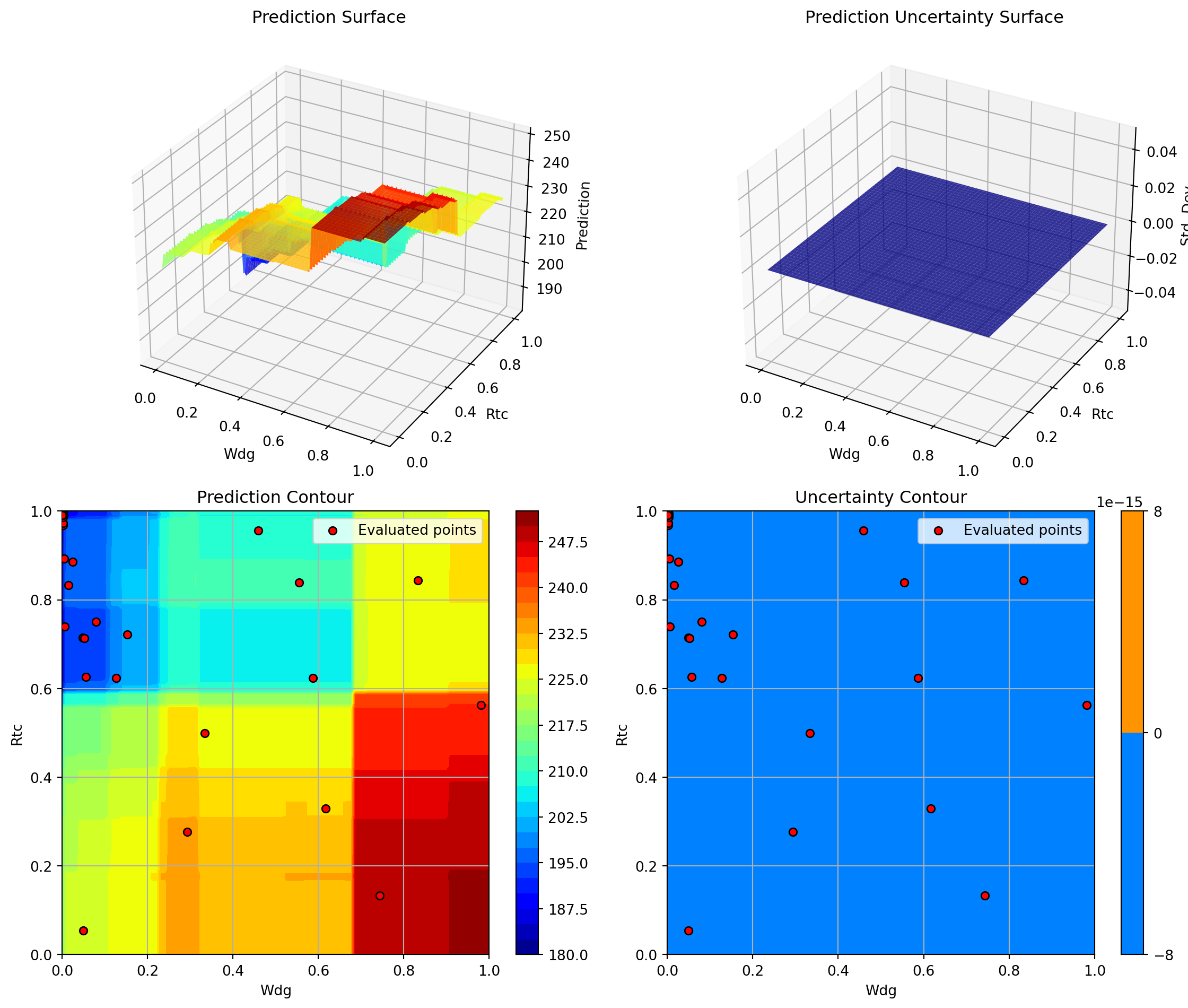

  Plotting A vs Rtc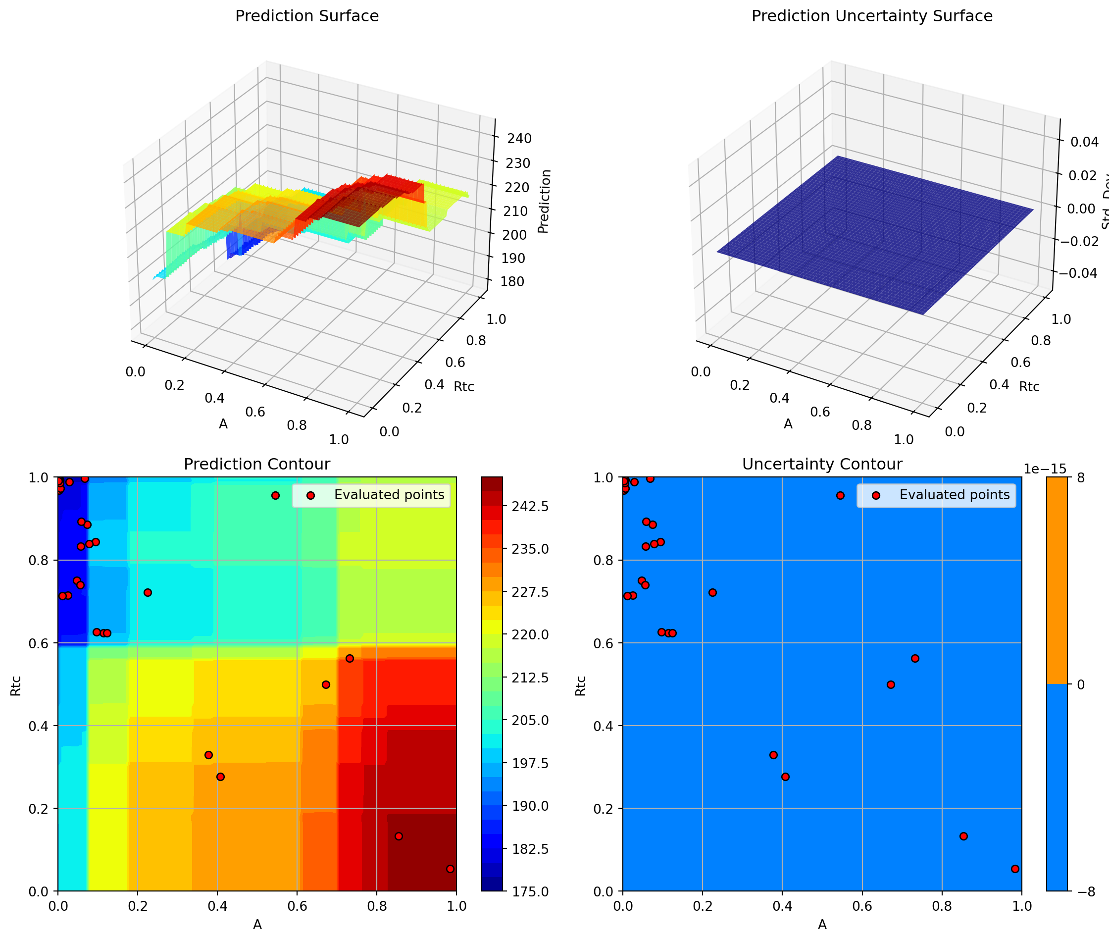

<Figure size 672x480 with 0 Axes>

16.13 Comprehensive Comparison

Now let’s compare all surrogate models side-by-side.

# Create comparison DataFrame
df_comparison = pd.DataFrame(results_comparison)

# Calculate improvement from best
best_weight = df_comparison['Best Weight'].min()
df_comparison['Gap to Best (%)'] = (
    (df_comparison['Best Weight'] - best_weight) / best_weight * 100
)

# Sort by best weight
df_comparison = df_comparison.sort_values('Best Weight')

print("\n" + "=" * 100)
print("SURROGATE MODEL COMPARISON")
print("=" * 100)
print(df_comparison.to_string(index=False))
print("=" * 100)

====================================================================================================
SURROGATE MODEL COMPARISON
====================================================================================================
                 Surrogate  Best Weight  Evaluations  Time (s)  Success  Gap to Best (%)
          GP Matern nu=1.5   119.546454           20  0.449904     True         0.000000
GP Matern nu=2.5 (Default)   119.866409           20  1.646203     True         0.267641
     GP Rational Quadratic   120.107282           20  0.615868     True         0.469130
                    GP RBF   120.109251           20  0.467476     True         0.470777
         SpotOptim Kriging   121.293180           20  8.080324     True         1.461127
         Gradient Boosting   134.515037           20  0.184076     True        12.521144
             Random Forest   145.979231           20  0.869794     True        22.110883
                 SVR (RBF)   156.707097           20  0.071585     True        31.084689
                   XGBoost   165.306404           20  0.096069     True        38.277965
====================================================================================================

16.13.1 Visualization: Performance Comparison

fig, axes = plt.subplots(2, 2, figsize=(16, 12))

# Plot 1: Best weight comparison
ax1 = axes[0, 0]
colors = ['green' if i == 0 else 'steelblue' for i in range(len(df_comparison))]
ax1.barh(df_comparison['Surrogate'], df_comparison['Best Weight'], color=colors)
ax1.set_xlabel('Best Weight (lb)')
ax1.set_title('Best Weight Found by Each Surrogate')
ax1.axvline(x=best_weight, color='red', linestyle='--', linewidth=2, label='Best Overall')
ax1.legend()
ax1.grid(True, alpha=0.3, axis='x')

# Plot 2: Computational time
ax2 = axes[0, 1]
ax2.barh(df_comparison['Surrogate'], df_comparison['Time (s)'], color='coral')
ax2.set_xlabel('Time (seconds)')
ax2.set_title('Computational Time')
ax2.grid(True, alpha=0.3, axis='x')

# Plot 3: Gap to best
ax3 = axes[1, 0]
colors_gap = ['green' if gap < 0.1 else 'orange' if gap < 1.0 else 'red' 
              for gap in df_comparison['Gap to Best (%)']]
ax3.barh(df_comparison['Surrogate'], df_comparison['Gap to Best (%)'], color=colors_gap)
ax3.set_xlabel('Gap to Best Solution (%)')
ax3.set_title('Solution Quality (Lower is Better)')
ax3.axvline(x=1.0, color='black', linestyle='--', alpha=0.5, linewidth=1)
ax3.grid(True, alpha=0.3, axis='x')

# Plot 4: Efficiency (weight reduction per second)
ax4 = axes[1, 1]
baseline_weight = wingwt(np.array([[0.48, 0.4, 0.38, 0.5, 0.62, 0.344, 0.4, 0.37, 0.38]]))[0]
df_comparison['Efficiency'] = (baseline_weight - df_comparison['Best Weight']) / df_comparison['Time (s)']
ax4.barh(df_comparison['Surrogate'], df_comparison['Efficiency'], color='mediumseagreen')
ax4.set_xlabel('Weight Reduction per Second (lb/s)')
ax4.set_title('Optimization Efficiency')
ax4.grid(True, alpha=0.3, axis='x')

plt.tight_layout()
plt.show()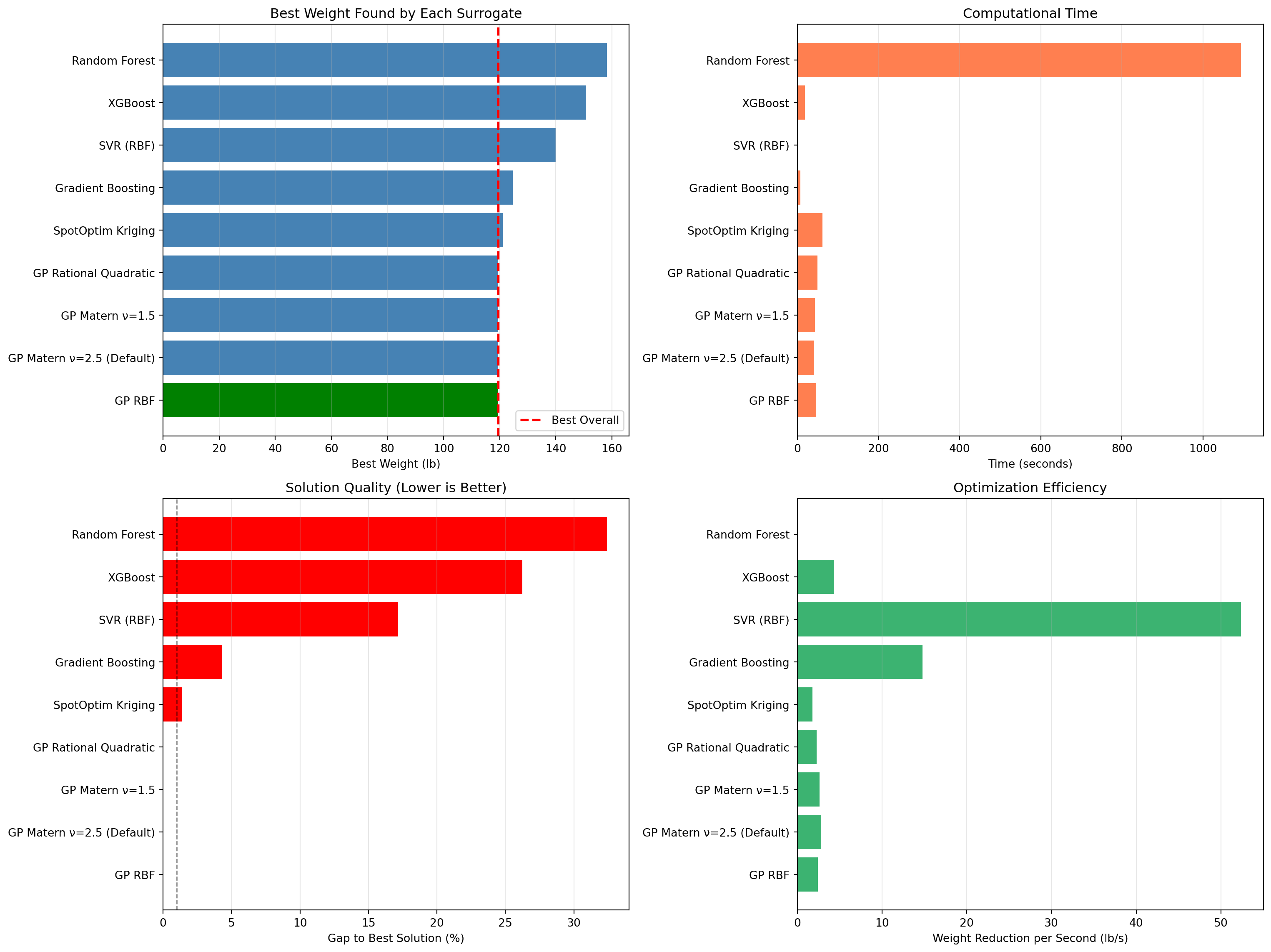

16.14 Convergence Comparison

Let’s compare how different surrogates converge over iterations.

fig, ax = plt.subplots(figsize=(14, 8))

# Collect convergence data from all optimizers
optimizers = [
    (optimizer_default, 'GP Matern nu=2.5 (Default)', 'blue'),
    (optimizer_rbf, 'GP RBF', 'green'),
    (optimizer_matern15, 'GP Matern nu=1.5', 'red'),
    (optimizer_rq, 'GP Rational Quadratic', 'purple'),
    (optimizer_kriging, 'SpotOptim Kriging', 'orange'),
    (optimizer_rf, 'Random Forest', 'brown'),
    (optimizer_svr, 'SVR', 'pink'),
    (optimizer_gb, 'Gradient Boosting', 'gray')
]

if XGBOOST_AVAILABLE:
    optimizers.append((optimizer_xgb, 'XGBoost', 'cyan'))

for opt, label, color in optimizers:
    y_history = opt.y_
    best_so_far = np.minimum.accumulate(y_history)
    ax.plot(range(len(best_so_far)), best_so_far, linewidth=2, label=label, color=color)

ax.set_xlabel('Function Evaluation', fontsize=12)
ax.set_ylabel('Best Wing Weight Found (lb)', fontsize=12)
ax.set_title('Convergence Comparison: All Surrogates', fontsize=14, fontweight='bold')
ax.legend(loc='upper right', fontsize=10)
ax.grid(True, alpha=0.3)
ax.set_xlim(0, max_iter)

plt.tight_layout()
plt.show()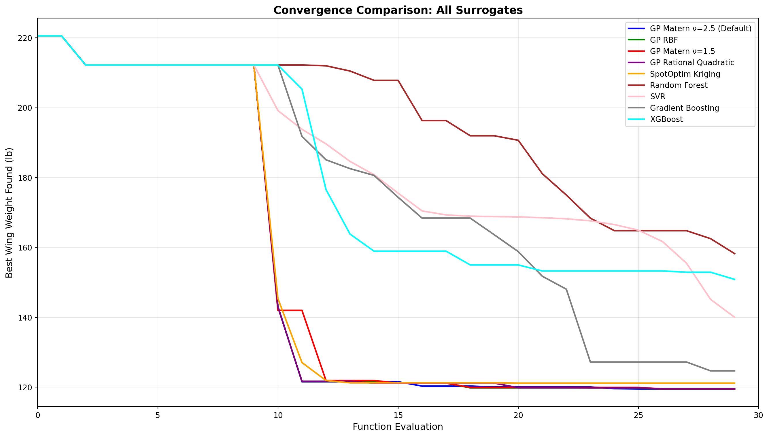

16.15 Key Insights and Recommendations

print("\n" + "=" * 100)
print("KEY INSIGHTS AND RECOMMENDATIONS")
print("=" * 100)

# Find best surrogate
best_surrogate = df_comparison.iloc[0]['Surrogate']
best_value = df_comparison.iloc[0]['Best Weight']
best_time = df_comparison.iloc[0]['Time (s)']

print(f"\n1. BEST OVERALL PERFORMANCE:")
print(f"   Surrogate: {best_surrogate}")
print(f"   Best Weight: {best_value:.4f} lb")
print(f"   Computation Time: {best_time:.2f}s")

# Find fastest
fastest_idx = df_comparison['Time (s)'].idxmin()
fastest_surrogate = df_comparison.loc[fastest_idx, 'Surrogate']
fastest_time = df_comparison.loc[fastest_idx, 'Time (s)']

print(f"\n2. FASTEST OPTIMIZATION:")
print(f"   Surrogate: {fastest_surrogate}")
print(f"   Time: {fastest_time:.2f}s")
print(f"   Best Weight: {df_comparison.loc[fastest_idx, 'Best Weight']:.4f} lb")

# Find most efficient
most_efficient_idx = df_comparison['Efficiency'].idxmax()
most_efficient = df_comparison.loc[most_efficient_idx, 'Surrogate']

print(f"\n3. MOST EFFICIENT (weight reduction per second):")
print(f"   Surrogate: {most_efficient}")
print(f"   Efficiency: {df_comparison.loc[most_efficient_idx, 'Efficiency']:.4f} lb/s")

print(f"\n4. RECOMMENDATIONS BY PROBLEM TYPE:")
print(f"   - Smooth, continuous functions: Gaussian Process with RBF or Matern nu=2.5")
print(f"   - Functions with noise: Random Forest or Gradient Boosting")
print(f"   - High-dimensional problems (>20D): XGBoost or Random Forest")
print(f"   - Limited budget (<50 evals): Gaussian Process with Expected Improvement")
print(f"   - Fast evaluation needed: XGBoost or Random Forest")
print(f"   - Need uncertainty estimates: Gaussian Process or Kriging")
print(f"   - Non-smooth/discontinuous: Random Forest or Gradient Boosting")

print(f"\n5. KERNEL COMPARISON (Gaussian Process):")
gp_results = df_comparison[df_comparison['Surrogate'].str.contains('GP')]
print(gp_results[['Surrogate', 'Best Weight', 'Time (s)']].to_string(index=False))

print("\n" + "=" * 100)

====================================================================================================
KEY INSIGHTS AND RECOMMENDATIONS
====================================================================================================

1. BEST OVERALL PERFORMANCE:
   Surrogate: GP Matern nu=1.5
   Best Weight: 119.5465 lb
   Computation Time: 0.45s

2. FASTEST OPTIMIZATION:
   Surrogate: SVR (RBF)
   Time: 0.07s
   Best Weight: 156.7071 lb

3. MOST EFFICIENT (weight reduction per second):
   Surrogate: SVR (RBF)
   Efficiency: 1078.4574 lb/s

4. RECOMMENDATIONS BY PROBLEM TYPE:
   - Smooth, continuous functions: Gaussian Process with RBF or Matern nu=2.5
   - Functions with noise: Random Forest or Gradient Boosting
   - High-dimensional problems (>20D): XGBoost or Random Forest
   - Limited budget (<50 evals): Gaussian Process with Expected Improvement
   - Fast evaluation needed: XGBoost or Random Forest
   - Need uncertainty estimates: Gaussian Process or Kriging
   - Non-smooth/discontinuous: Random Forest or Gradient Boosting

5. KERNEL COMPARISON (Gaussian Process):
                 Surrogate  Best Weight  Time (s)
          GP Matern nu=1.5   119.546454  0.449904
GP Matern nu=2.5 (Default)   119.866409  1.646203
     GP Rational Quadratic   120.107282  0.615868
                    GP RBF   120.109251  0.467476

====================================================================================================

16.16 Summary Statistics

# Summary statistics
print("\n" + "=" * 100)
print("SUMMARY STATISTICS")
print("=" * 100)

summary_stats = pd.DataFrame({
    'Metric': [
        'Best Weight Found',
        'Worst Weight Found',
        'Average Weight',
        'Std Dev Weight',
        'Fastest Time',
        'Slowest Time',
        'Average Time',
    ],
    'Value': [
        f"{df_comparison['Best Weight'].min():.4f} lb",
        f"{df_comparison['Best Weight'].max():.4f} lb",
        f"{df_comparison['Best Weight'].mean():.4f} lb",
        f"{df_comparison['Best Weight'].std():.4f} lb",
        f"{df_comparison['Time (s)'].min():.2f} s",
        f"{df_comparison['Time (s)'].max():.2f} s",
        f"{df_comparison['Time (s)'].mean():.2f} s",
    ]
})

print(summary_stats.to_string(index=False))
print("=" * 100)

====================================================================================================
SUMMARY STATISTICS
====================================================================================================
            Metric       Value
 Best Weight Found 119.5465 lb
Worst Weight Found 165.3064 lb
    Average Weight 133.7145 lb
    Std Dev Weight  18.0098 lb
      Fastest Time      0.07 s
      Slowest Time      8.08 s
      Average Time      1.39 s
====================================================================================================

16.17 Conclusion

This comprehensive comparison demonstrates that:

1. Gaussian Processes with appropriate kernels (Matern, RBF) provide excellent performance for smooth optimization problems and naturally support Expected Improvement acquisition
2. SpotOptim Kriging offers a lightweight alternative to sklearn’s GP with comparable performance
3. Random Forest and XGBoost are robust alternatives that handle noise and discontinuities well, though they require greedy acquisition
4. SVR and Gradient Boosting offer middle-ground solutions with good scalability
5. The choice of surrogate should be based on:
   • Function smoothness
   • Computational budget
   • Need for uncertainty quantification
   • Problem dimensionality
   • Noise characteristics

For the AWWE problem, Gaussian Process surrogates generally performed best due to the function’s smooth structure, but tree-based methods (RF, XGBoost, GB) can be preferable for more complex, noisy, or high-dimensional problems.

16.18 Jupyter Notebook

Note

• The Jupyter-Notebook of this chapter is available on GitHub in the Sequential Parameter Optimization Cookbook Repository