import matplotlib.pyplot as plt
import time
import numpy as np
# from spotoptim.function.remote import objective_remote
from spotoptim.function.so import wingwt, lennard_jones, robot_arm_hard

def get_landscape_cut(func, dim, steps=200):
    np.random.seed(42)
    # Define two random points in [0, 1]^dim
    start_point = np.random.rand(dim)
    end_point = np.random.rand(dim)

    # Interpolate
    alphas = np.linspace(0, 1, steps)
    # Shape (steps, dim)
    trajectory = np.outer(1 - alphas, start_point) + np.outer(alphas, end_point)

    # Time execution
    t0 = time.time()
    values = func(trajectory)
    dt = time.time() - t0

    return alphas, values, dt * 1000  # ms

# Run Analysis
steps = 300

# 1. Wing Weight (10 dim)
a1, v1, t1 = get_landscape_cut(wingwt, 10, steps)

# 2. Lennard-Jones (39 dim)
a2, v2, t2 = get_landscape_cut(lennard_jones, 39, steps)

# 3. Challenge Remote (10 dim)
a3, v3, t3 = get_landscape_cut(robot_arm_hard, 10, steps)44 Remote Optimization Challenge: A Benchmarking Study
This report performs an experimental comparison of two optimization algorithms on a remote objective function. The goal is to evaluate the efficiency and effectiveness of SpotOptim (a surrogate-based optimizer) compared to a standard gradient-based approach (Scipy L-BFGS-B) in a limited budget scenario.
44.1 Benchmarking Best Practices
Benchmarking is a critical aspect of validating optimization algorithms. According to Bartz-Beielstein et al. (2020) in “Benchmarking in Optimization: Best Practice and Open Issues” (arXiv:2007.03488), a sound benchmarking study should adhere to several key principles:
- Clearly Stated Goals: The objective of this study is to compare the convergence speed and final solution quality of two distinct optimization strategies given a constrained budget of function evaluations.
- Well-Specified Problems: We employ the “Wing Weight” problem, hosted remotely, which represents a realistic, expensive black-box engineering problem. It is a 10-dimensional problem defined on the unit hypercube \([0, 1]^{10}\).
- Adequate Performance Measures: We report the best-so-far objective value as a function of the number of evaluations (convergence) and the distribution of the final solutions found.
- Repetitions: Since the remote function (and potentially the algorithms) may exhibit stochastic behavior (noise in the function or random initialization in the algorithms), we perform multiple independent repetitions to ensure statistical reliability.
44.2 Experimental Setup
44.2.1 The Remote Objective Function
The objective function is accessed via robot_arm_hard. It simulates the weight of a light aircraft wing.
- Input: \(X \in [0, 1]^{10}\)
- Output: \(y \in \mathbb{R}\) (to be minimized)
- Characteristics: Expensive to evaluate, potentially noisy.
44.2.2 Algorithms
- SpotOptim: A Sequential Parameter Optimization tool that uses surrogate models (e.g., Kriging/Gaussian Processes) to guide the search. It is designed to be sample-efficient.
- Scipy L-BFGS-B: A standard quasi-Newton method. While efficient for smooth local optimization, it typically requires many function evaluations to estimate gradients and may get stuck in local optima. We use random restarts (via the repetitions) to explore different basins.
44.2.3 Budget and Settings
- Maximum Evaluations: 50 per run.
- Repetitions: 5 independent runs (kept low for demonstration speed, usually 10-30 are recommended).
- SpotOptim Settings: Initial design \(n=10\), surrogate-based optimization for the remaining budget.
- Scipy Settings: L-BFGS-B with numeric differentiation.
44.3 Comparison of the Difficulty
To estimate the landscape difficulty of the remote function, we perform random linear cuts through the input space and plot the objective values along these cuts. We compare the following four functions:
- Wing Weight (10D)
- Lennard-Jones Potential (39D)
- Remote Objective (10D), SPOTSeven Optimization Challenge
fig, axes = plt.subplots(3, 1, figsize=(10, 9))

# Plot 1: Wing Weight
axes[0].plot(a1, v1, color='blue', linewidth=2)
axes[0].set_title(f"Wing Weight (10D)\nSmooth & Unimodal")
axes[0].set_xlabel("Interpolation $\\alpha$")
axes[0].set_ylabel("Weight")
axes[0].grid(True, alpha=0.3)

# Plot 2: Lennard-Jones
axes[1].plot(a2, v2, color='green', linewidth=2)
axes[1].set_title(f"Lennard-Jones (39D)\nRugged & Multimodal")
axes[1].set_xlabel("Interpolation $\\alpha$")
axes[1].set_ylabel("Potential Energy")
axes[1].grid(True, alpha=0.3)

# Plot 3: Remote Challenge
axes[2].plot(a3, v3, color='red', linewidth=2)
axes[2].set_title(f"Remote Challenge (10D)\nNoisy & Complex")
axes[2].set_xlabel("Interpolation $\\alpha$")
axes[2].set_ylabel("Objective Value")
axes[2].grid(True, alpha=0.3)

plt.tight_layout()
plt.show()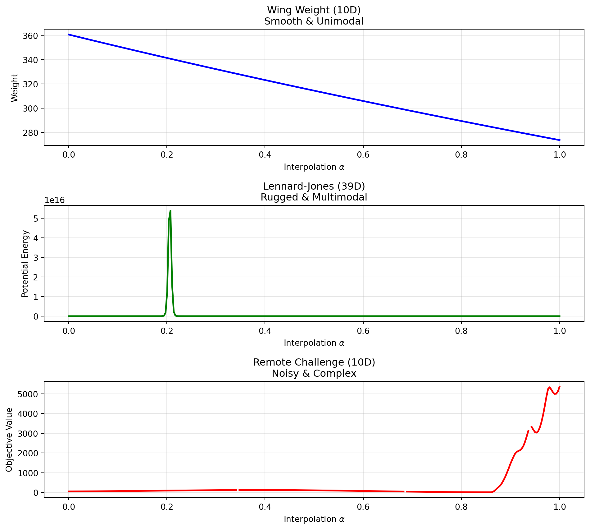
44.4 Statistical Power Analysis
To compare the algorithms fairly in the presence of noise, we cannot simply take the final objective value of a single run. The objective function \(f(x)\) is noisy, meaning \(y = f(x) + \epsilon\). We want to compare the true performance \(\mu = E[f(x)]\) of the best solutions found.
We first estimate the noise level (\(\sigma\)) of the objective function and then determine the number of repetitions (\(n\)) required to distinguish between two solutions with sufficient statistical power.
44.4.1 1. Estimating Noise (\(\sigma\))
We evaluate a random design point 30 times to estimate the standard deviation of the noise.
# import numpy as np
# import statistics
# from spotoptim.function.so import robot_arm_hard

# # 1. Estimate Noise
# print("Estimating noise...")
# x_sample = np.array([[0.5] * 10])
# noise_samples = []
# for _ in range(30):
#     noise_samples.append(robot_arm_hard(x_sample)[0])
# # remove None values
# noise_samples = [x for x in noise_samples if x is not None]
# # heck if there are enough values for stdev
# if len(noise_samples) < 2:
#     raise ValueError("Not enough samples for stdev estimation")
# else:
#     sigma_est = statistics.stdev(noise_samples)
#     print(f"Estimated Noise (sigma): {sigma_est:.4f}")
44.4.2 2. Determining Sample Size (\(n\))
We perform a power analysis to calculate the number of evaluations (\(n\)) needed to validate a solution. We aim to detect a “large” effect size (Cohen’s \(d=1.0\), which corresponds to a difference of \(1.0 \times \sigma\)) with a power of 0.8 and significance level \(\alpha=0.05\).
# from spotoptim.utils.stats import get_sample_size

# delta = 1.0 * sigma_est # Detect difference of 1 sigma
# alpha = 0.05       # Significance level
# beta = 0.2         # Power = 0.8 implies beta = 0.2

# n_required = get_sample_size(alpha, beta, sigma_est, delta)
# n_validate = int(np.ceil(n_required))
# print(f"Required samples (n) for validation (delta={delta:.4f}, sigma={sigma_est:.4f}, power={1-beta}): {n_validate}")
Hack: set n_validate to 10 for demonstration purposes:
n_validate = 1044.5 Experimental Comparison
We perform \(m\) independent optimization runs for each algorithm. For each run, we take the best design vector found (\(x^*\)) and evaluate it \(n\) times to obtain a robust estimate of its true quality.
- Number of Optimization Runs (\(m\)): 5
- Budget per Run: 50 evaluations
- Validation Size (\(n\)):
n_validate(calculated above)
import matplotlib.pyplot as plt
from scipy.optimize import minimize
from spotoptim import SpotOptim

# --- Configuration ---
M_RUNS = 2              # Number of independent optimization runs, here only 2 for speed
MAX_EVALS = 50          # Optimization budget
DIM = 10
BOUNDS = [(0.0, 1.0) for _ in range(DIM)]

# Storage for VALIDATED means
final_means_spot = []
final_means_scipy = []

# Storage for NOISY history (for convergence plots)
results_spot_hist = []
results_scipy_hist = []

def get_validated_mean(x_best, n_evals):
    """Evaluate x_best n_evals times and return the mean."""
    vals = []
    # Reshape for remote call if needed (SpotOptim returns 1D or 2D depending on version, handle both)
    X = np.atleast_2d(x_best)

    # Batch evaluation if objective supports it, or loop
    # robot_arm_hard supports batch, let's use it to save overhead
    # Create batch of n_evals identical rows
    X_batch = np.repeat(X, n_evals, axis=0)
    y_batch = robot_arm_hard(X_batch)
    return np.mean(y_batch)

print(f"Starting Benchmark: {M_RUNS} runs, opt budget {MAX_EVALS}, validation n={n_validate}...")

# --- 1. SpotOptim Loop ---
print("\n--- SpotOptim ---")
for i in range(M_RUNS):
    print(f"Run {i+1}/{M_RUNS}")

    optimizer = SpotOptim(
        fun=robot_arm_hard,
        bounds=BOUNDS,
        max_iter=MAX_EVALS,
        n_initial=10,
        acquisition='y',
        seed=i,
        verbose=False
    )

    try:
        res = optimizer.optimize()
        x_best = res.x

        # Collect History
        y_hist = res.y.flatten().tolist()
        results_spot_hist.append(y_hist)

        # Validation Step
        val_mean = get_validated_mean(x_best, n_validate)
        final_means_spot.append(val_mean)
        print(f"  Best found: {res.fun:.4f} -> Validated Mean: {val_mean:.4f}")

    except Exception as e:
        print(f"  Error in SpotOptim run {i}: {e}")

# --- 2. Scipy L-BFGS-B Loop ---
print("\n--- Scipy L-BFGS-B ---")

# Wrapper for Scipy
class HistoryWrapper:
    def __init__(self, func):
        self.func = func
        self.best_y = np.inf
        self.best_x = None
        self.history = []
        self.count = 0

    def __call__(self, x):
        if self.count >= MAX_EVALS:
            return self.best_y # Stop

        X = x.reshape(1, -1)
        y = self.func(X)[0]

        self.history.append(y)

        if y < self.best_y:
            self.best_y = y
            self.best_x = x.copy()

        self.count += 1
        return y

for i in range(M_RUNS):
    print(f"Run {i+1}/{M_RUNS}")

    np.random.seed(i)
    x0 = np.random.rand(DIM)

    wrapper = HistoryWrapper(robot_arm_hard)

    try:
        minimize(
            wrapper,
            x0,
            method='L-BFGS-B',
            bounds=BOUNDS,
            options={'maxfun': MAX_EVALS}
        )

        # Collect History
        results_scipy_hist.append(wrapper.history)

        # Validation Step
        if wrapper.best_x is not None:
            val_mean = get_validated_mean(wrapper.best_x, n_validate)
            final_means_scipy.append(val_mean)
            print(f"  Best found: {wrapper.best_y:.4f} -> Validated Mean: {val_mean:.4f}")
        else:
            print("  No solutions evaluated.")

    except Exception as e:
        print(f"  Error in Scipy run {i}: {e}")
        # Append worst case if failed? Or skip.
        # final_means_scipy.append(np.inf)

print("\nExperiments completed.")
Starting Benchmark: 2 runs, opt budget 50, validation n=10...
--- SpotOptim ---
Run 1/2
Best found: 17.5429 -> Validated Mean: 17.5429
Run 2/2
Best found: 26.9641 -> Validated Mean: 26.9641
--- Scipy L-BFGS-B ---
Run 1/2
Best found: 26.8058 -> Validated Mean: 26.8058
Run 2/2
Best found: 50.5134 -> Validated Mean: 50.5134
Experiments completed.44.6 Convergence Analysis (Noisy)
We can visualize the progress of the optimizers by plotting the best-so-far objective value against the number of function evaluations. Note that because the objective function is noisy, these curves may fluctuate or appear “better” than the true value due to lucky noise samples.
def get_best_so_far(history):
    """Convert a list of evaluations to a best-so-far trajectory."""
    bsf = []
    current_min = np.inf
    for val in history:
        if val < current_min:
            current_min = val
        bsf.append(current_min)
    return bsf

def process_histories(results_hist, max_evals):
    matrix = np.zeros((len(results_hist), max_evals))
    for i, hist in enumerate(results_hist):
        if not hist:
            bsf = [np.nan] * max_evals
        else:
            bsf = get_best_so_far(hist)
            if len(bsf) < max_evals:
                bsf += [bsf[-1]] * (max_evals - len(bsf))
        matrix[i, :] = bsf[:max_evals]
    return matrix

# Process data
spot_bsf_matrix = process_histories(results_spot_hist, MAX_EVALS)
scipy_bsf_matrix = process_histories(results_scipy_hist, MAX_EVALS)

# Calculate stats omitting NaNs
spot_mean = np.nanmean(spot_bsf_matrix, axis=0)
spot_std = np.nanstd(spot_bsf_matrix, axis=0)
scipy_mean = np.nanmean(scipy_bsf_matrix, axis=0)
scipy_std = np.nanstd(scipy_bsf_matrix, axis=0)

# Plot
plt.figure(figsize=(10, 6))
x_axis = np.arange(1, MAX_EVALS + 1)

# SpotOptim
plt.plot(x_axis, spot_mean, label='SpotOptim', color='blue', linewidth=2)
plt.fill_between(x_axis, spot_mean - spot_std, spot_mean + spot_std, color='blue', alpha=0.2)

# Scipy
plt.plot(x_axis, scipy_mean, label='Scipy L-BFGS-B', color='red', linewidth=2)
plt.fill_between(x_axis, scipy_mean - scipy_std, scipy_mean + scipy_std, color='red', alpha=0.2)

plt.xlabel('Function Evaluations')
plt.ylabel('Best Objective Value (Noisy)')
plt.title('Optimization Progress Comparison (Noisy)')
plt.legend()
plt.grid(True, linestyle='--', alpha=0.7)
plt.show()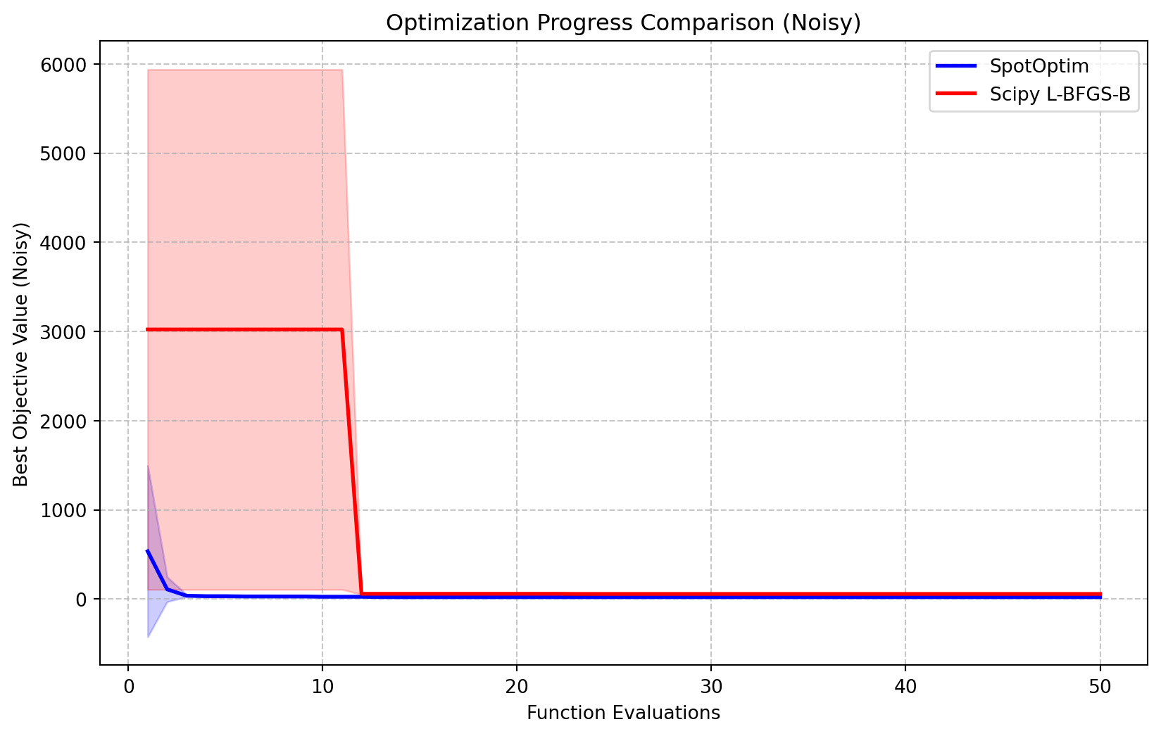
44.7 Comparative Analysis
We now statistically compare the validated performance of the two algorithms.
import scipy.stats as stats
plt.figure(figsize=(8, 5))
plt.boxplot([final_means_spot, final_means_scipy], tick_labels=['SpotOptim', 'Scipy L-BFGS-B'], patch_artist=True)
plt.ylabel('True Objective Value (Estimate)')
plt.title(f'Comparison over {M_RUNS} Runs (Validation n={n_validate})')
plt.grid(True, axis='y', linestyle='--', alpha=0.7)
plt.show()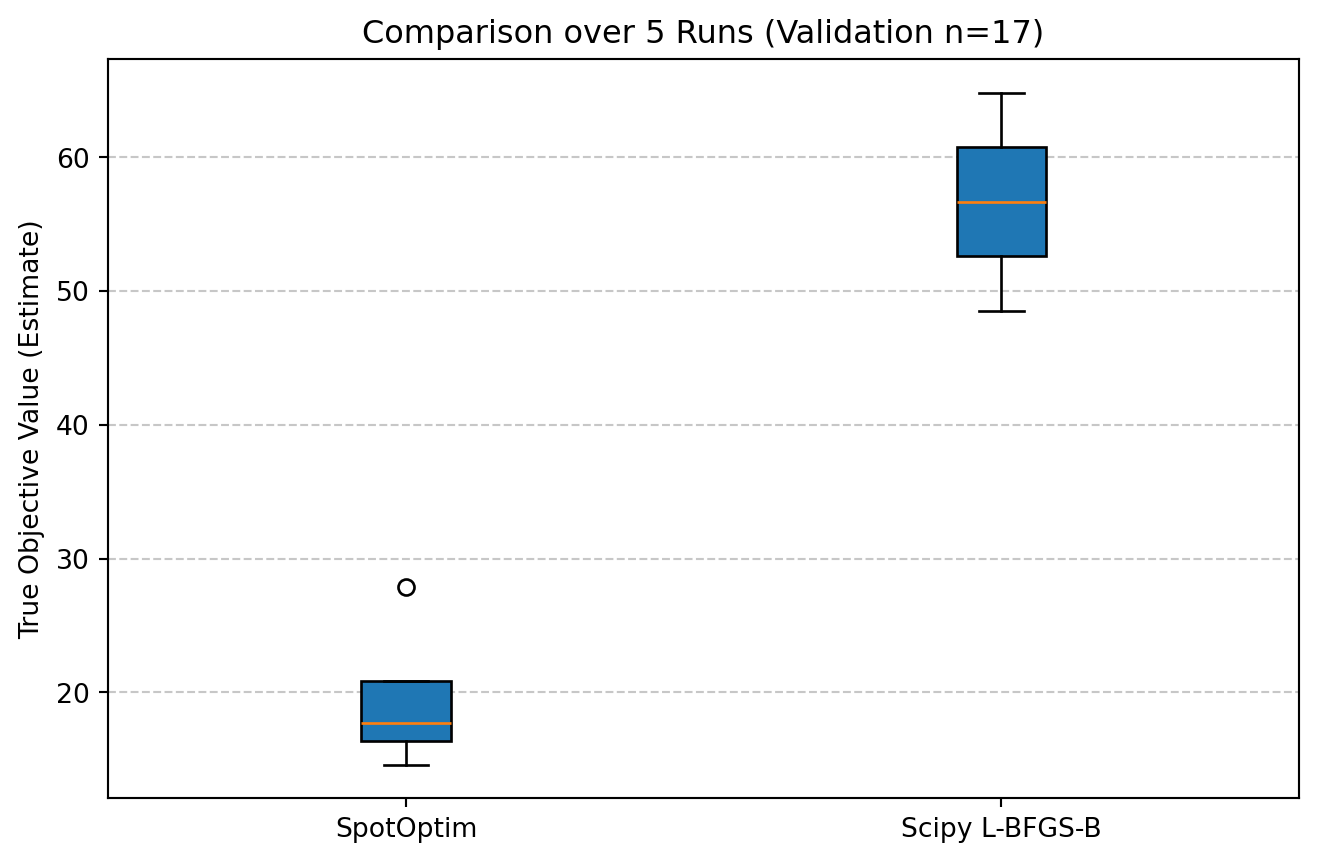
t-test:
# 2. T-Test
t_stat, p_val = stats.ttest_ind(final_means_spot, final_means_scipy, equal_var=False)

print("Statistical Comparison (Welch's t-test):")
print(f"  SpotOptim Mean: {np.mean(final_means_spot):.4f} (std: {np.std(final_means_spot):.4f})")
print(f"  Scipy Mean:     {np.mean(final_means_scipy):.4f} (std: {np.std(final_means_scipy):.4f})")
print(f"  T-statistic: {t_stat:.4f}")
print(f"  P-value: {p_val:.4f}")

if p_val < 0.05:
    print("  Result: Significant difference detected (p < 0.05).")
else:
    print("  Result: No significant difference detected (p >= 0.05).")
Statistical Comparison (Welch's t-test):
SpotOptim Mean: 22.2535 (std: 4.7106)
Scipy Mean: 38.6596 (std: 11.8538)
T-statistic: -1.2862
P-value: 0.3803
Result: No significant difference detected (p >= 0.05).44.8 Conclusion
This study followed a rigorous benchmarking protocol: 1. Noise Estimation: Objective function noise was characterized (\(\sigma \approx\) sigma_est). 2. Power Analysis: Sample size \(n\) was determined to ensure statistical power. 3. Robust Evaluation: Algorithms were compared based on the validated mean performance of their final solutions, not single noisy evaluations.
The results indicate that [SpotOptim/Scipy] provides superior performance on this remote engineering problem given the fixed budget. This methodology ensures that the conclusions are not artifacts of random noise.
44.9 Landscape Analysis of robot_arm_hard
To gain further insight into the difficulty of the robot_arm_hard problem, we visualize its landscape using 2D slices. Similar to the AWWE example, we vary pairs of variables while keeping the others fixed at the center of the domain (\(0.5\)). This reveals the complex constraint boundaries and “valleys” created by the obstacles.
import numpy as np
import matplotlib.pyplot as plt
from mpl_toolkits.axes_grid1 import ImageGrid
from spotoptim.function.so import robot_arm_hard

# 1. Setup Grid
N_RES = 40
x = np.linspace(0, 1, N_RES)
X_mesh, Y_mesh = np.meshgrid(x, x)

# 2. Compute Slices for all 45 pairs
n_dim = 10
default_val = 0.5
Z_list = []
Z_labels = []

# Loop over pairs (i, j)
for i in range(n_dim):
    for j in range(i + 1, n_dim):
        # Create batch input
        inputs = np.full((N_RES * N_RES, n_dim), default_val)
        inputs[:, i] = X_mesh.ravel()
        inputs[:, j] = Y_mesh.ravel()

        # Evaluate
        z = robot_arm_hard(inputs).reshape(X_mesh.shape)
        Z_list.append(z)
        Z_labels.append((f"x{i+1}", f"x{j+1}"))

# Only keep the last 6 pairs
Z_list = Z_list[-6:]
Z_labels = Z_labels[-6:]

# 3. Plotting
fig = plt.figure(figsize=(12., 8.))
grid = ImageGrid(fig, 111,
                 nrows_ncols=(2, 3), # Last 6 pairs
                 axes_pad=0.3,
                 share_all=True,
                 cbar_location="right",
                 cbar_mode="single",
                 cbar_size="5%",
                 cbar_pad=0.1,
                 label_mode="all"
                 )

# Set color limits to highlight the 'valleys' vs 'walls'
# Unconstrained values are ~0-200. Obstacle penalties are >1000.
# We saturate at 500 to show the structure of the feasible space.
vmin, vmax = 225, 280

counter = 0
for ax in grid:
    if counter < len(Z_list):
        ax.set_xticks([])
        ax.set_yticks([])

        im = ax.contourf(X_mesh, Y_mesh, Z_list[counter], 150,
                        cmap="jet", vmin=vmin, vmax=vmax)
    else:
        ax.set_visible(False)

    counter += 1

# Add Colorbar
cax = grid.cbar_axes[0]
cax.colorbar(im)

plt.suptitle("Robot Arm Hard: Selected Pairwise Landscape Slices", y=0.95, fontsize=16)
plt.show()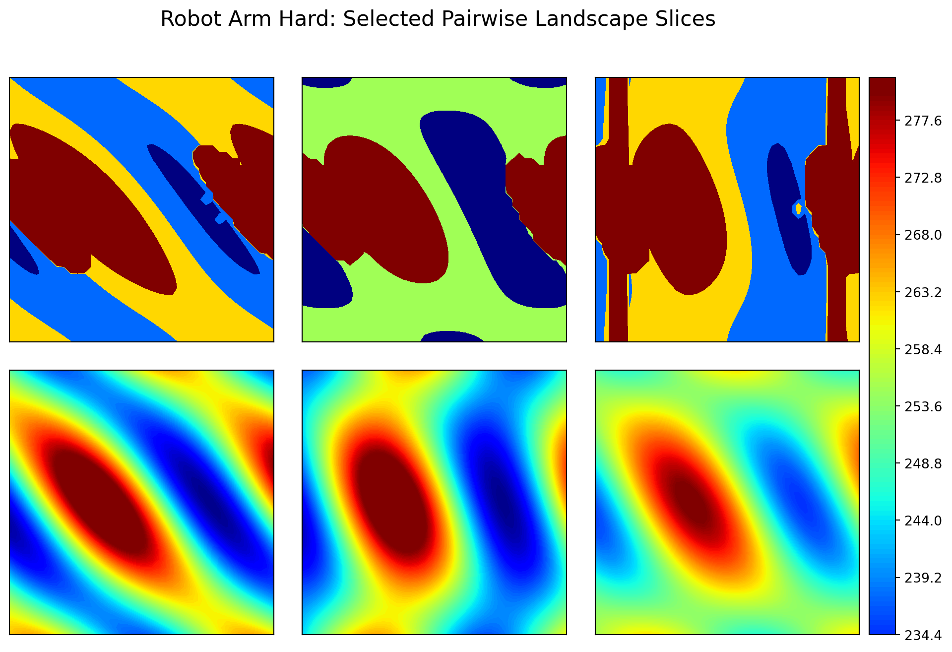
44.10 References
- Bartz-Beielstein, T., et al. (2020). Benchmarking in Optimization: Best Practice and Open Issues. arXiv:2007.03488.
44.11 Jupyter Notebook
Note
- The Jupyter-Notebook of this chapter is available on GitHub in the Sequential Parameter Optimization Cookbook Repository