This tutorial demonstrates how to use Physics-Informed Neural Networks (PINNs) to solve ordinary differential equations (ODEs) using SpotOptim’s LinearRegressor class. We’ll solve a first-order ODE with an initial condition, combining data-driven learning with physics constraints.
import matplotlib.pyplot as pltimport numpy as npimport torchimport torch.nn as nnfrom typing import Tuplefrom spotoptim.nn.linear_regressor import LinearRegressor# Set random seed for reproducibilitytorch.manual_seed(123)
<torch._C.Generator at 0x1168e7730>
30 The Neural Network
We’ll use SpotOptim’s LinearRegressor class to create a neural network with:
1 input (time t)
1 output (solution y)
32 neurons per hidden layer
3 hidden layers
Tanh activation function
model = LinearRegressor( input_dim=1, output_dim=1, l1=32, num_hidden_layers=3, activation="Tanh", lr=1.0)# Get optimizer with custom learning rateoptimizer = model.get_optimizer("Adam", lr=3.0) # 3.0 * 0.001 = 0.003print(f"Model architecture:")print(model)
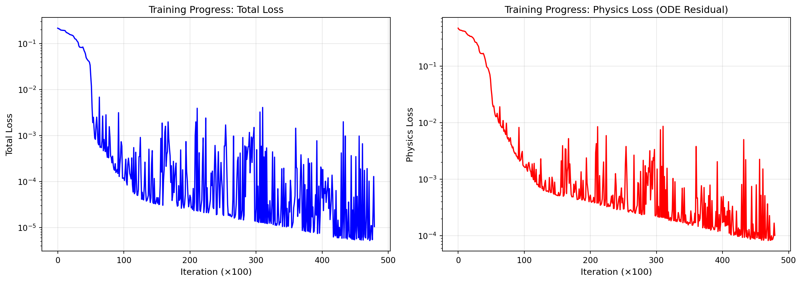
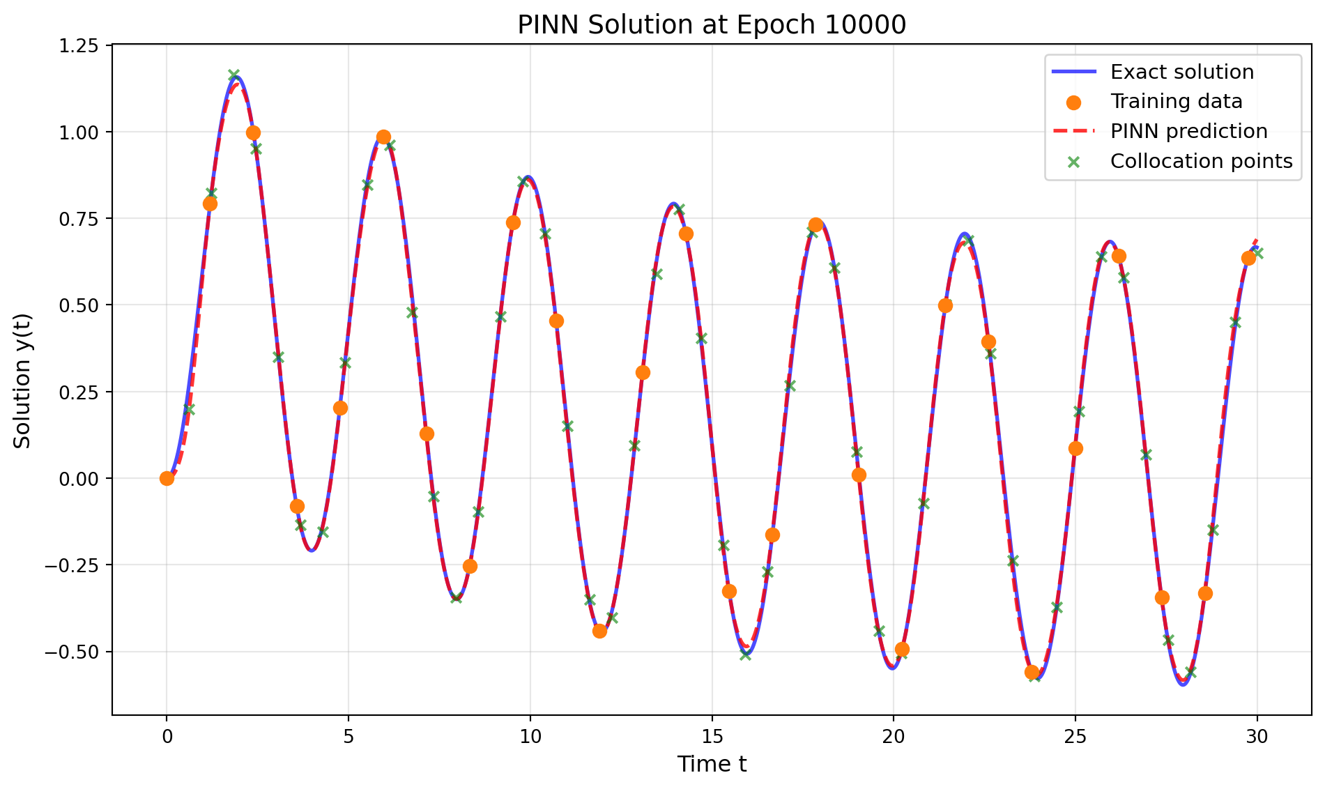
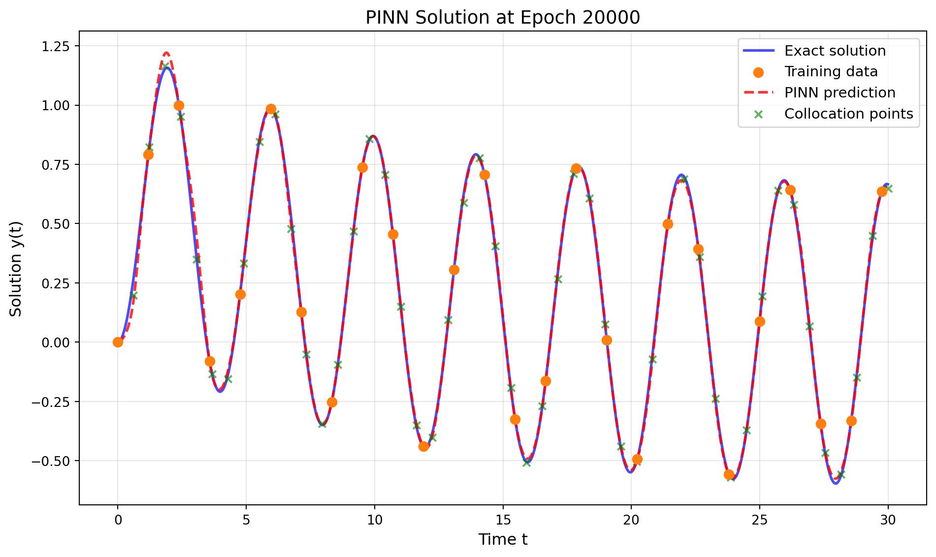
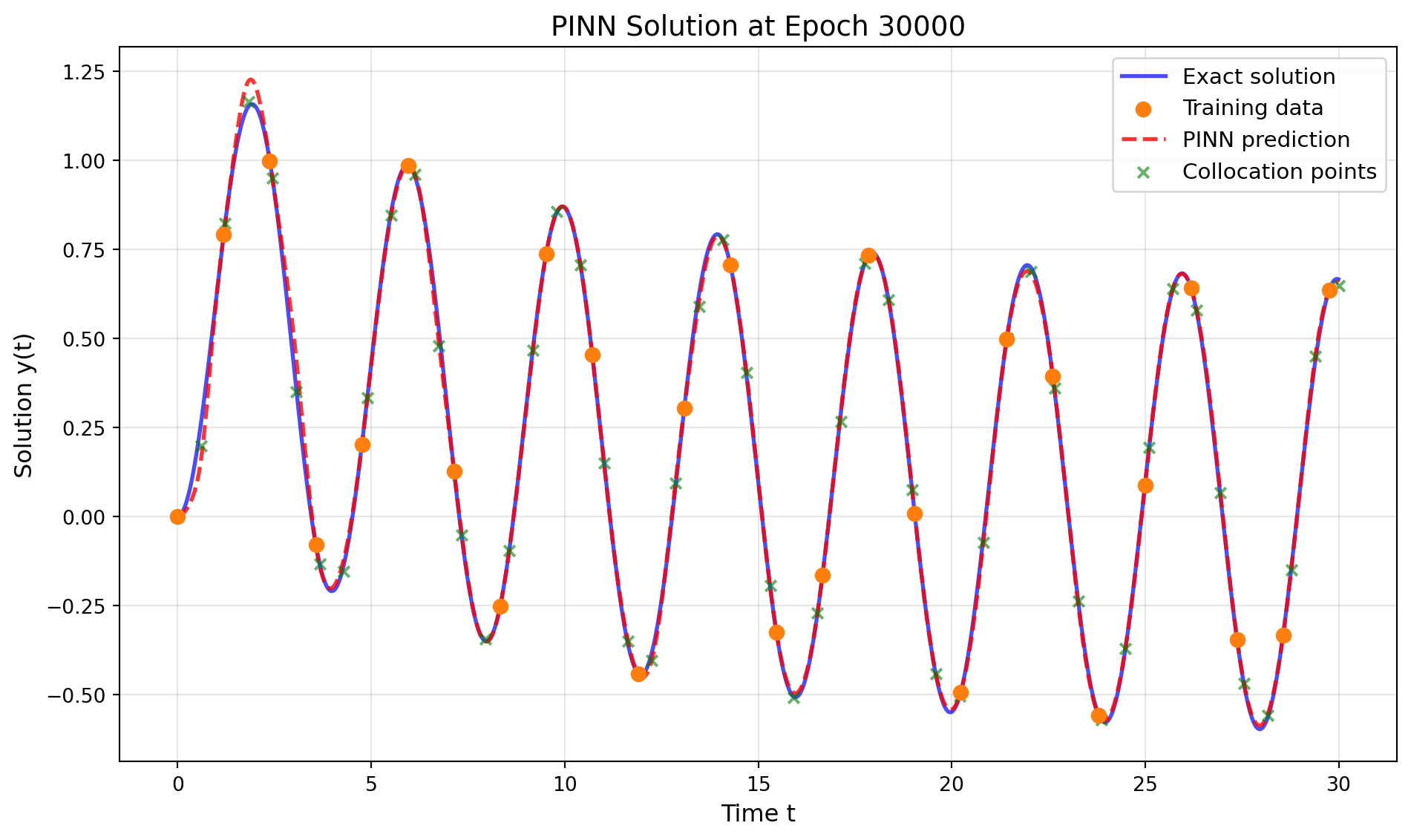
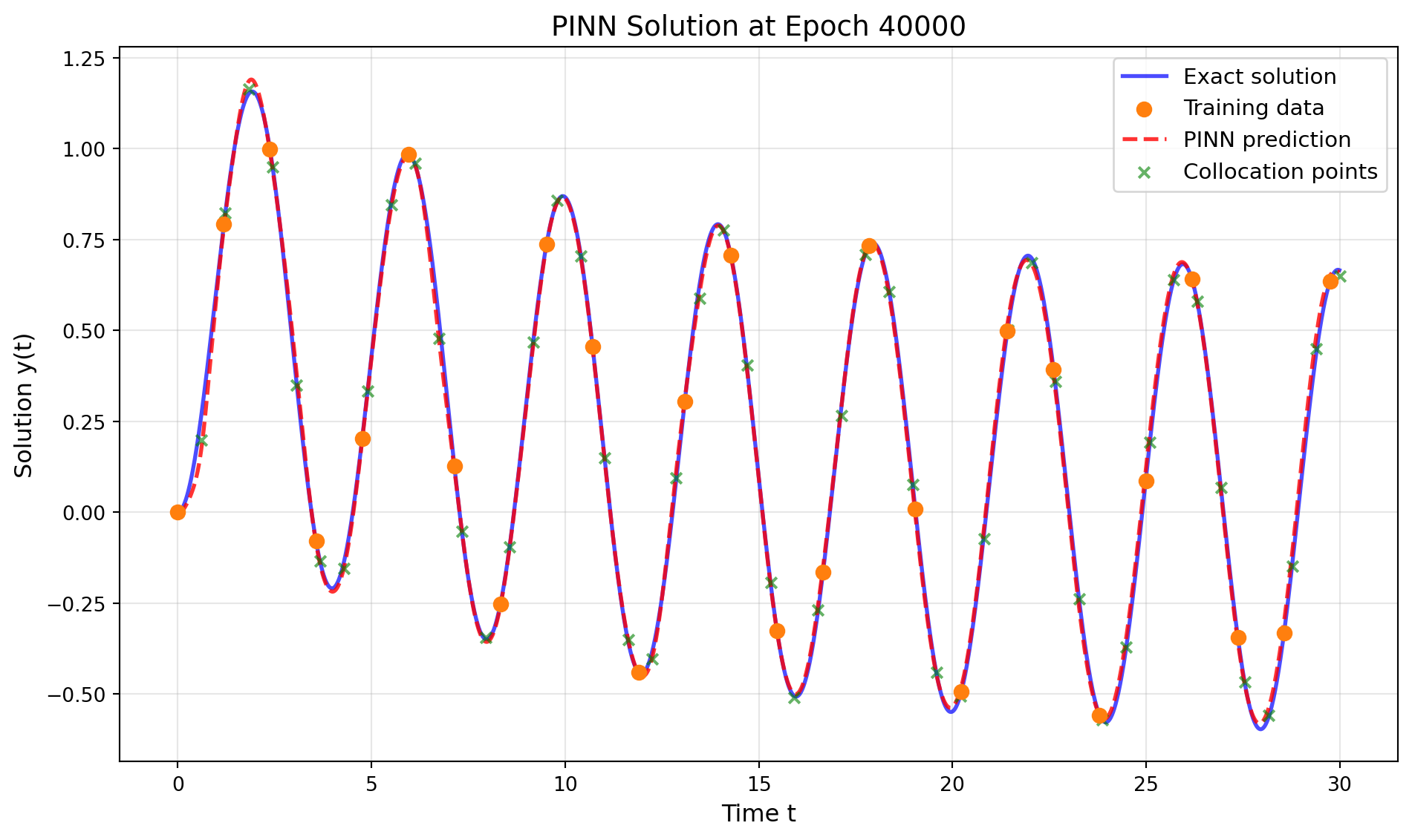
loss_history_pinn = []loss2_history_pinn = []plot_data_points_pinn = []alpha =6e-2# Weight for physics lossn_epochs =48000print("Training Physics-Informed Neural Network...")print(f"Total epochs: {n_epochs}")print(f"Physics loss weight (alpha): {alpha}")for i inrange(n_epochs): optimizer.zero_grad()# Data Loss: Fit the training data yh = model(x_data) loss1 = torch.mean((yh - y_data)**2)# Physics Loss: Satisfy the ODE at collocation points yhp = model(x_physics) dyhp_dxphysics = torch.autograd.grad( yhp, x_physics, torch.ones_like(yhp), create_graph=True )[0] physics = dyhp_dxphysics +0.1* yhp - torch.sin(np.pi * x_physics /2) loss2 = torch.mean(physics**2)# Total Loss loss = loss1 + alpha * loss2 loss.backward() optimizer.step()# Store history every 100 stepsif (i +1) %100==0: loss_history_pinn.append(loss.detach()) loss2_history_pinn.append(loss2.detach())# Store snapshots for visualization every 10000 stepsif (i +1) %10000==0: current_yh_full = model(x).detach() plot_data_points_pinn.append({'yh': current_yh_full, 'step': i +1 })print(f"Epoch {i+1}/{n_epochs}: Total Loss = {loss.item():.6f}, "f"Physics Loss = {loss2.item():.6f}")print("Training completed!")
Training Physics-Informed Neural Network...
Total epochs: 48000
Physics loss weight (alpha): 0.06
Epoch 10000/48000: Total Loss = 0.000321, Physics Loss = 0.002949
Epoch 20000/48000: Total Loss = 0.000020, Physics Loss = 0.000309
Epoch 30000/48000: Total Loss = 0.000095, Physics Loss = 0.000285
Epoch 40000/48000: Total Loss = 0.000823, Physics Loss = 0.001919
Training completed!
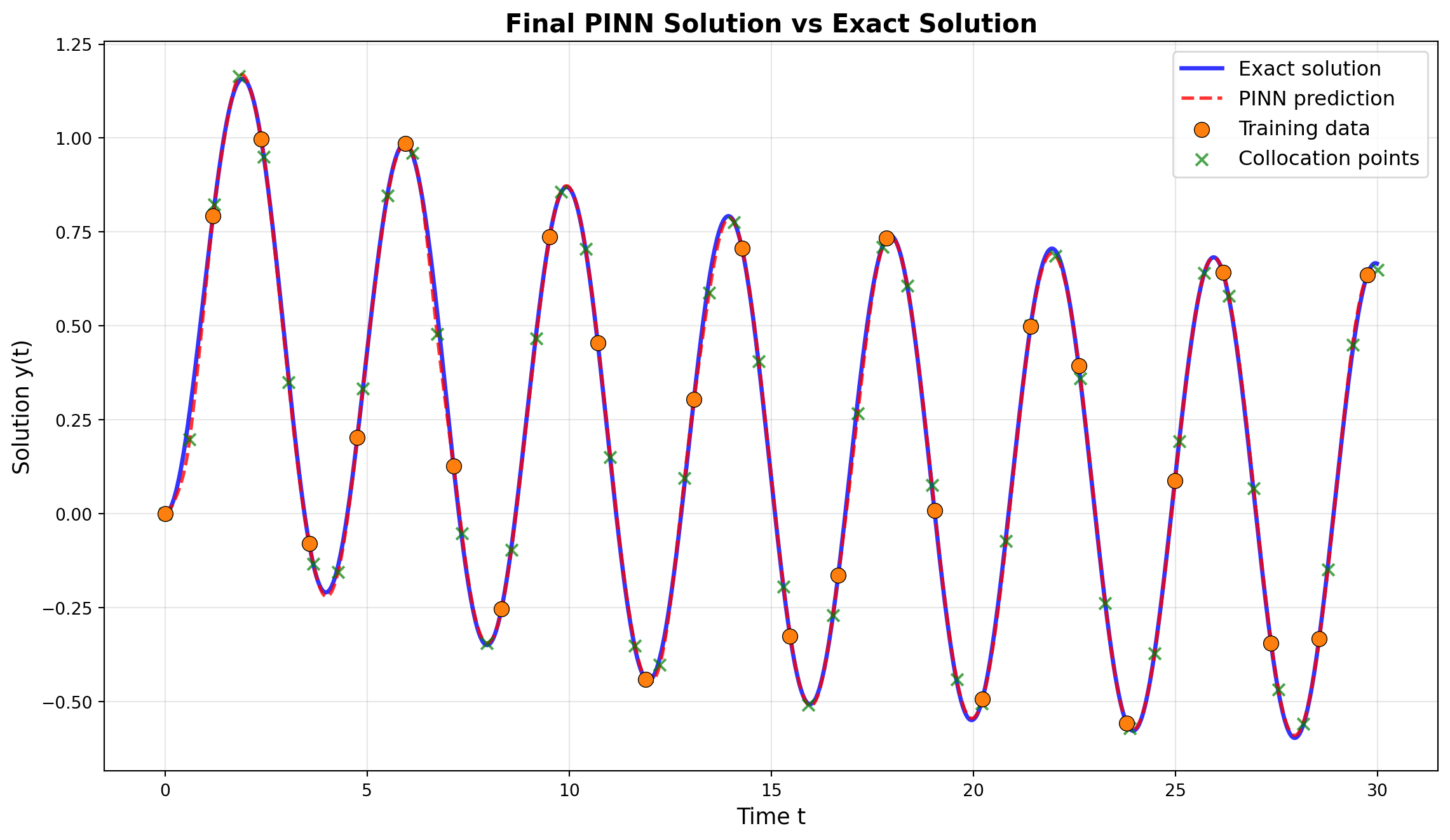
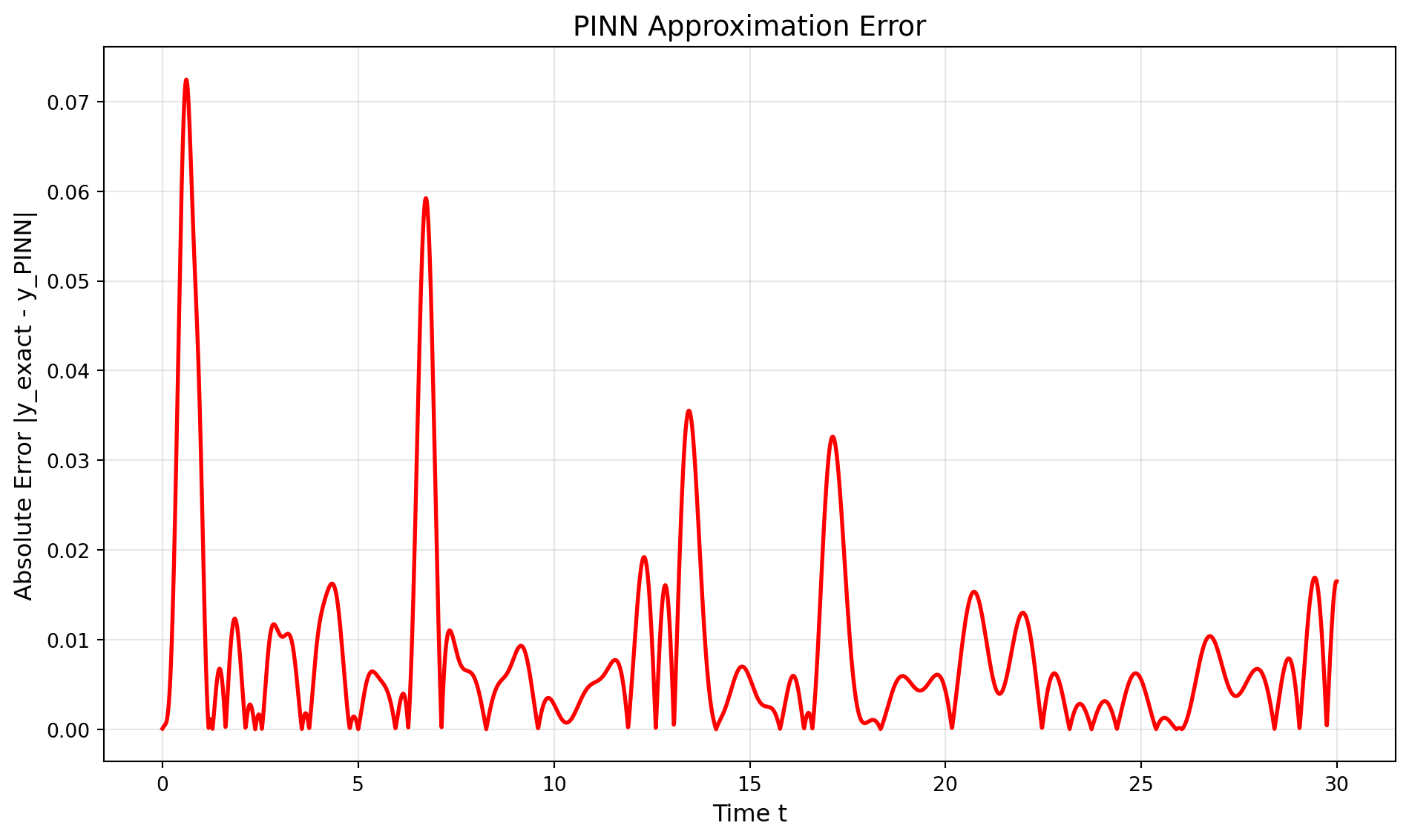
Error Statistics:
Maximum absolute error: 0.125975
Mean absolute error: 0.010835
Root mean squared error: 0.021054
35 Summary
This tutorial demonstrated how to use SpotOptim’s LinearRegressor class to implement a Physics-Informed Neural Network (PINN) for solving ordinary differential equations. Key takeaways:
Network Architecture: Used a 3-layer neural network with 32 neurons per layer and Tanh activation
Dual Loss Function: Combined data fitting loss with physics constraint loss
Automatic Differentiation: Leveraged PyTorch’s autograd to compute derivatives for the ODE
Collocation Method: Enforced the ODE at specific points in the domain
Training Strategy: Balanced data-driven and physics-informed learning with weight α
The PINN successfully learned to approximate the ODE solution using only sparse training data (~25 points) by incorporating the underlying physics through the differential equation constraint.
35.1 Key Advantages of PINNs
Data Efficiency: Can learn with very few data points
Physics Consistency: Solutions automatically satisfy the governing equations
Generalization: Better extrapolation beyond training data
Flexibility: Can handle complex geometries and boundary conditions
35.2 Using SpotOptim for Hyperparameter Optimization
The LinearRegressor class integrates seamlessly with SpotOptim for hyperparameter tuning:
from spotoptim import SpotOptimdef train_pinn(X):"""Objective function for hyperparameter optimization.""" results = []for params in X: l1 =int(params[0]) # Hidden layer size num_layers =int(params[1]) # Number of layers lr_unified =10** params[2] # Learning rate (log scale)# Create model model = LinearRegressor( input_dim=1, output_dim=1, l1=l1, num_hidden_layers=num_layers, activation="Tanh", lr=lr_unified )# Train PINN and compute validation error# ... training code ... results.append(validation_error)return np.array(results)# Optimize hyperparametersoptimizer = SpotOptim( fun=train_pinn, bounds=[(16, 128), (1, 5), (-4, 0)], var_type=["int", "int", "float"], var_name=["layer_size", "num_layers", "log_lr"], max_iter=50)result = optimizer.optimize()
This approach allows you to systematically find the best network architecture and learning rate for your specific PINN problem.