import numpy as np
import matplotlib.pyplot as plt
import pandas as pd
from scipy.optimize import minimize
from spotoptim import SpotOptim
import time
import pprint4 Optimizing the Aircraft Wing Weight Example
NoteNote
- This section demonstrates optimization of the Aircraft Wing Weight Example (AWWE) function
- We compare three optimization methods:
- SpotOptim: Bayesian optimization with Gaussian Process surrogate
- Nelder-Mead: Derivative-free simplex method from scipy.optimize
- BFGS: Quasi-Newton method from scipy.optimize
- The following Python packages are imported:
4.1 The AWWE Objective Function
We use the same AWWE function from Chapter 34, which models the weight of an unpainted light aircraft wing. The function accepts inputs in the unit cube \([0,1]^9\) and returns the wing weight.
def wingwt(x):
    """
    Aircraft Wing Weight function.

    Args:
        x: array-like of 9 values in [0,1]
           [Sw, Wfw, A, L, q, l, Rtc, Nz, Wdg]

    Returns:
        Wing weight (scalar)
    """
    # Ensure x is a 2D array for batch evaluation
    x = np.atleast_2d(x)

    # Transform from unit cube to natural scales
    Sw = x[:, 0] * (200 - 150) + 150
    Wfw = x[:, 1] * (300 - 220) + 220
    A = x[:, 2] * (10 - 6) + 6
    L = (x[:, 3] * (10 - (-10)) - 10) * np.pi/180
    q = x[:, 4] * (45 - 16) + 16
    l = x[:, 5] * (1 - 0.5) + 0.5
    Rtc = x[:, 6] * (0.18 - 0.08) + 0.08
    Nz = x[:, 7] * (6 - 2.5) + 2.5
    Wdg = x[:, 8] * (2500 - 1700) + 1700

    # Calculate weight on natural scale
    W = 0.036 * Sw**0.758 * Wfw**0.0035 * (A/np.cos(L)**2)**0.6 * q**0.006
    W = W * l**0.04 * (100*Rtc/np.cos(L))**(-0.3) * (Nz*Wdg)**(0.49)

    return W.ravel()


# Wrapper for scipy.optimize (expects 1D input, returns scalar)
def wingwt_scipy(x):
    return float(wingwt(x.reshape(1, -1))[0])
4.2 Baseline Configuration
The baseline Cessna C172 Skyhawk configuration (coded in unit cube):
baseline_coded = np.array([0.48, 0.4, 0.38, 0.5, 0.62, 0.344, 0.4, 0.37, 0.38])
baseline_weight = wingwt(baseline_coded)[0]
print(f"Baseline wing weight: {baseline_weight:.2f} lb")
Baseline wing weight: 233.91 lb4.3 Optimization Setup
We’ll optimize the AWWE function starting from the baseline configuration using three different methods:
- SpotOptim: Bayesian optimization (good for expensive black-box functions)
- Nelder-Mead: Derivative-free simplex method (robust but can be slow)
- BFGS: Quasi-Newton method (fast but requires smooth functions)
# Starting point (baseline configuration)
x0 = baseline_coded.copy()

# Bounds for all methods (unit cube)
bounds = [(0, 1)] * 9

# Number of function evaluations budget
max_evals = 30

print(f"Starting point: {x0}")
print(f"Starting weight: {baseline_weight:.2f} lb")
Starting point: [0.48 0.4 0.38 0.5 0.62 0.344 0.4 0.37 0.38 ]
Starting weight: 233.91 lb4.4 Method 1: SpotOptim (Surrogate Model Based Optimization)
# Start timing
start_time = time.time()

# Configure SpotOptim
optimizer_spot = SpotOptim(
    fun=wingwt,
    bounds=bounds,
    x0=None,
    max_iter=max_evals,
    n_initial=10,  # Initial design points
    var_name=['Sw', 'Wfw', 'A', 'L', 'q', 'l', 'Rtc', 'Nz', 'Wdg'],
    acquisition='y',  # ei: Expected Improvement
    max_surrogate_points=100,
    seed=42,
    verbose=True,
    tensorboard_log=True,
    tensorboard_clean=True
)
Removed old TensorBoard logs: runs/spotoptim_20260701_193805
Cleaned 1 old TensorBoard log directory
TensorBoard logging enabled: runs/spotoptim_20260701_2018134.5 Design Table
pprint.pprint(optimizer_spot.get_design_table())('| name | type | lower | upper | default | transform |\n'
'|--------|--------|---------|---------|-----------|-------------|\n'
'| Sw | float | 0 | 1 | 0.5 | - |\n'
'| Wfw | float | 0 | 1 | 0.5 | - |\n'
'| A | float | 0 | 1 | 0.5 | - |\n'
'| L | float | 0 | 1 | 0.5 | - |\n'
'| q | float | 0 | 1 | 0.5 | - |\n'
'| l | float | 0 | 1 | 0.5 | - |\n'
'| Rtc | float | 0 | 1 | 0.5 | - |\n'
'| Nz | float | 0 | 1 | 0.5 | - |\n'
'| Wdg | float | 0 | 1 | 0.5 | - |')4.6 Run optimization
result_spot = optimizer_spot.optimize()Initial best: f(x) = 205.911302
Iter 1 | Best: 205.911302 | Curr: 207.213032 | Rate: 0.00 | Evals: 36.7%
Iter 2 | Best: 123.245058 | Rate: 0.50 | Evals: 40.0%
Iter 3 | Best: 123.050044 | Rate: 0.67 | Evals: 43.3%
Iter 4 | Best: 122.581938 | Rate: 0.75 | Evals: 46.7%
Iter 5 | Best: 121.850820 | Rate: 0.80 | Evals: 50.0%
Iter 6 | Best: 121.742699 | Rate: 0.83 | Evals: 53.3%
Iter 7 | Best: 121.577343 | Rate: 0.86 | Evals: 56.7%
Iter 8 | Best: 120.643326 | Rate: 0.88 | Evals: 60.0%
Iter 9 | Best: 120.013506 | Rate: 0.89 | Evals: 63.3%
Iter 10 | Best: 119.701481 | Rate: 0.90 | Evals: 66.7%
Iter 11 | Best: 119.506129 | Rate: 0.91 | Evals: 70.0%
Iter 12 | Best: 119.503886 | Rate: 0.92 | Evals: 73.3%
Iter 13 | Best: 119.503673 | Rate: 0.92 | Evals: 76.7%
Iter 14 | Best: 119.503673 | Curr: 119.503677 | Rate: 0.86 | Evals: 80.0%
Iter 15 | Best: 119.503672 | Rate: 0.87 | Evals: 83.3%
Iter 16 | Best: 119.503672 | Curr: 119.503777 | Rate: 0.81 | Evals: 86.7%
Iter 17 | Best: 119.503672 | Curr: 119.503814 | Rate: 0.76 | Evals: 90.0%
Iter 18 | Best: 119.503672 | Curr: 119.504008 | Rate: 0.72 | Evals: 93.3%
Iter 19 | Best: 119.503672 | Curr: 119.503679 | Rate: 0.68 | Evals: 96.7%
Iter 20 | Best: 119.503672 | Curr: 119.503672 | Rate: 0.65 | Evals: 100.0%
TensorBoard writer closed. View logs with: tensorboard --logdir=runs/spotoptim_20260701_201813# End timing
spot_time = time.time() - start_time
print(f"\nSpotOptim Results:")
print(f" Best weight: {result_spot.fun:.4f} lb")
print(f" Function evaluations: {result_spot.nfev}")
print(f" Time elapsed: {spot_time:.2f} seconds")
print(f" Success: {result_spot.success}")
SpotOptim Results:
  Best weight: 119.5037 lb
  Function evaluations: 30
  Time elapsed: 7.02 seconds
  Success: True
optimizer_spot.print_best()
Best Solution Found:
--------------------------------------------------
  Sw: 0.0000
  Wfw: 0.0000
  A: 0.0000
  L: 0.4999
  q: 0.0000
  l: 0.0000
  Rtc: 1.0000
  Nz: 0.0000
  Wdg: 0.0000
  Objective Value: 119.5037
  Total Evaluations: 30
4.7 Result Table
pprint.pprint(optimizer_spot.get_results_table(show_importance=True))('| name | type | default | lower | upper | tuned | transform '
'| importance | stars |\n'
'|--------|--------|-----------|---------|---------|---------|-------------|--------------|---------|\n'
'| Sw | float | 0.5 | 0 | 1 | 0 | - '
'| 12.79 | . |\n'
'| Wfw | float | 0.5 | 0 | 1 | 0 | - '
'| 14.41 | . |\n'
'| A | float | 0.5 | 0 | 1 | 0 | - '
'| 14.97 | . |\n'
'| L | float | 0.5 | 0 | 1 | 0.4999 | - '
'| 0.82 | |\n'
'| q | float | 0.5 | 0 | 1 | 0 | - '
'| 8.29 | |\n'
'| l | float | 0.5 | 0 | 1 | 0 | - '
'| 6.77 | |\n'
'| Rtc | float | 0.5 | 0 | 1 | 1 | - '
'| 13.06 | . |\n'
'| Nz | float | 0.5 | 0 | 1 | 0 | - '
'| 15.11 | . |\n'
'| Wdg | float | 0.5 | 0 | 1 | 0 | - '
'| 13.78 | . |\n'
'\n'
'Interpretation: ***: >99%, **: >75%, *: >50%, .: >10%')4.8 Progress of the Optimization
optimizer_spot.plot_progress(log_y=False)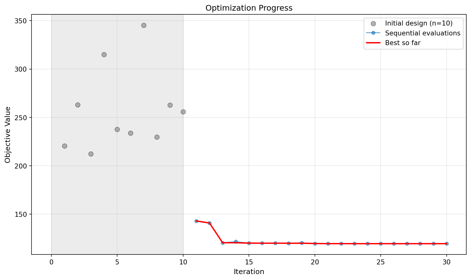
4.9 Contour Plots of Most Important Hyperparameters
optimizer_spot.plot_important_hyperparameter_contour(max_imp=3)Plotting surrogate contours for top 3 most important parameters:
Nz: importance = 15.11% (type: float)
A: importance = 14.97% (type: float)
Wfw: importance = 14.41% (type: float)
Generating 3 surrogate plots...
Plotting Nz vs A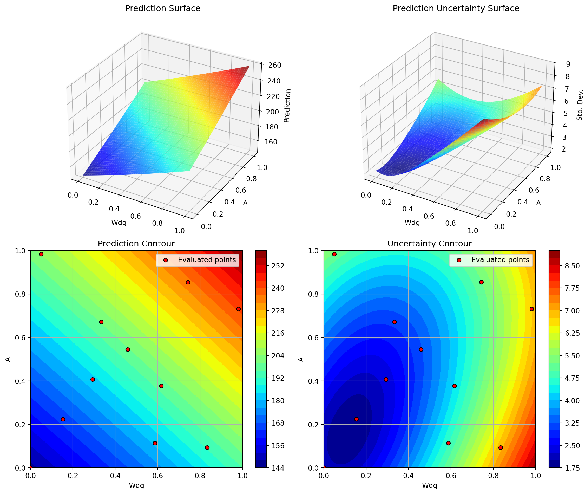
Plotting Nz vs Wfw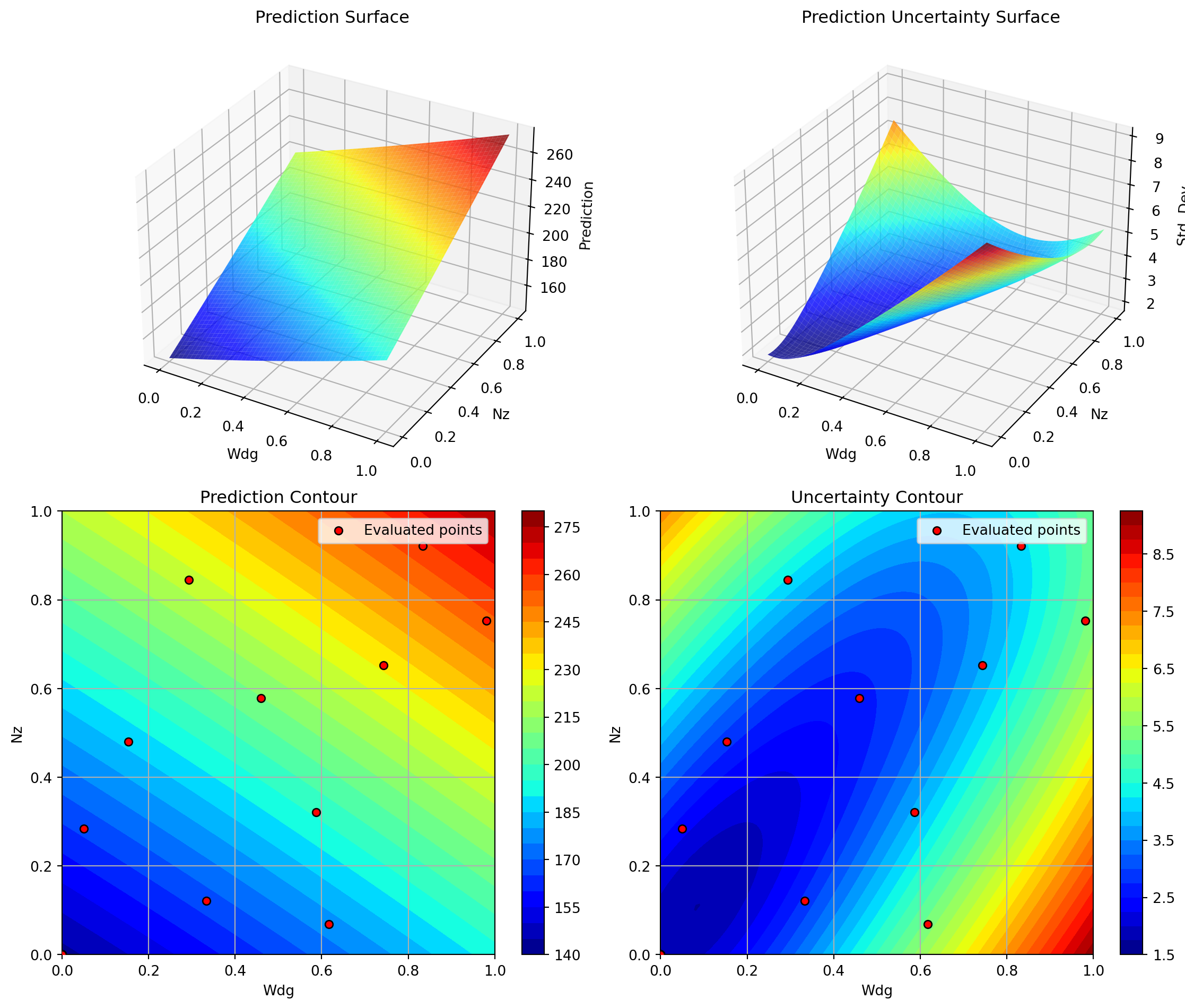
Plotting A vs Wfw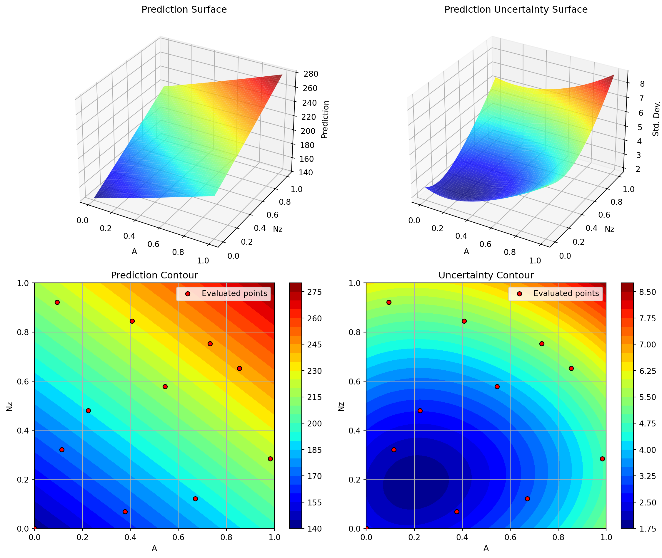
4.10 Method 2: Nelder-Mead Simplex
print("\n" + "=" * 60)
print("Running Nelder-Mead Simplex...")
print("=" * 60)

# Start timing
start_time = time.time()

# Run optimization
result_nm = minimize(
    wingwt_scipy,
    x0=x0,
    method='Nelder-Mead',
    bounds=bounds,
    options={'maxfev': max_evals, 'disp': True}
)

# End timing
nm_time = time.time() - start_time

print(f"\nNelder-Mead Results:")
print(f"  Best weight: {result_nm.fun:.4f} lb")
print(f"  Function evaluations: {result_nm.nfev}")
print(f"  Time elapsed: {nm_time:.2f} seconds")
print(f"  Success: {result_nm.success}")
============================================================
Running Nelder-Mead Simplex...
============================================================

Nelder-Mead Results:
  Best weight: 220.5449 lb
  Function evaluations: 30
  Time elapsed: 0.00 seconds
  Success: False
4.11 Method 3: BFGS (Quasi-Newton)
print("\n" + "=" * 60)
print("Running BFGS (Quasi-Newton)...")
print("=" * 60)


# Start timing
start_time = time.time()

# Run optimization
result_bfgs = minimize(
    wingwt_scipy,
    x0=x0,
    method='L-BFGS-B',  # Bounded BFGS
    bounds=bounds,
    options={'maxfun': max_evals, 'disp': True}
)

# End timing
bfgs_time = time.time() - start_time

print(f"\nBFGS Results:")
print(f"  Best weight: {result_bfgs.fun:.4f} lb")
print(f"  Function evaluations: {result_bfgs.nfev}")
print(f"  Time elapsed: {bfgs_time:.2f} seconds")
print(f"  Success: {result_bfgs.success}")
============================================================
Running BFGS (Quasi-Newton)...
============================================================

BFGS Results:
  Best weight: 119.5037 lb
  Function evaluations: 60
  Time elapsed: 0.00 seconds
  Success: False
4.12 Comparison of Results
# Create comparison DataFrame
comparison = pd.DataFrame({
    'Method': ['Baseline', 'SpotOptim', 'Nelder-Mead', 'BFGS'],
    'Best Weight (lb)': [
        baseline_weight,
        result_spot.fun,
        result_nm.fun,
        result_bfgs.fun
    ],
    'Improvement (%)': [
        0.0,
        (baseline_weight - result_spot.fun) / baseline_weight * 100,
        (baseline_weight - result_nm.fun) / baseline_weight * 100,
        (baseline_weight - result_bfgs.fun) / baseline_weight * 100
    ],
    'Function Evals': [
        1,
        result_spot.nfev,
        result_nm.nfev,
        result_bfgs.nfev
    ],
    'Time (s)': [
        0.0,
        spot_time,
        nm_time,
        bfgs_time
    ],
    'Success': [
        True,
        result_spot.success,
        result_nm.success,
        result_bfgs.success
    ]
})

print("\n" + "=" * 80)
print("OPTIMIZATION COMPARISON")
print("=" * 80)
print(comparison.to_string(index=False))
print("=" * 80)
================================================================================
OPTIMIZATION COMPARISON
================================================================================
     Method  Best Weight (lb)  Improvement (%)  Function Evals  Time (s)  Success
   Baseline        233.908405         0.000000               1  0.000000     True
  SpotOptim        119.503672        48.910057              30  7.019096     True
Nelder-Mead        220.544928         5.713124              30  0.000753    False
       BFGS        119.503672        48.910057              60  0.001350    False
================================================================================
4.13 Visualization: Convergence Plots
4.13.1 SpotOptim Convergence
fig, (ax1, ax2) = plt.subplots(1, 2, figsize=(14, 5))

# Plot 1: Best value over iterations
y_history = optimizer_spot.y_
best_so_far = np.minimum.accumulate(y_history)

ax1.plot(range(len(y_history)), y_history, 'o', alpha=0.5, label='Evaluated points')
ax1.plot(range(len(best_so_far)), best_so_far, 'r-', linewidth=2, label='Best so far')
ax1.axhline(y=baseline_weight, color='g', linestyle='--', label='Baseline')
ax1.set_xlabel('Function Evaluation')
ax1.set_ylabel('Wing Weight (lb)')
ax1.set_title('SpotOptim Convergence')
ax1.legend()
ax1.grid(True, alpha=0.3)

# Plot 2: Improvement over baseline
improvement = (baseline_weight - best_so_far) / baseline_weight * 100
ax2.plot(range(len(improvement)), improvement, 'b-', linewidth=2)
ax2.set_xlabel('Function Evaluation')
ax2.set_ylabel('Improvement over Baseline (%)')
ax2.set_title('SpotOptim Improvement Progress')
ax2.grid(True, alpha=0.3)
ax2.axhline(y=0, color='k', linestyle='-', alpha=0.3)

plt.tight_layout()
plt.show()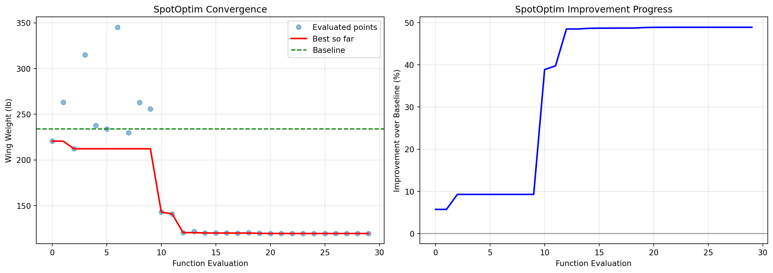
4.14 Optimal Parameter Values
Let’s examine the optimal parameter values found by each method:
# Parameter names
param_names = ['Sw', 'Wfw', 'A', 'L', 'q', 'l', 'Rtc', 'Nz', 'Wdg']

# Transform from unit cube to natural scales
def decode_params(x):
    scales = [
        (150, 200),      # Sw
        (220, 300),      # Wfw
        (6, 10),         # A
        (-10, 10),       # L (degrees)
        (16, 45),        # q
        (0.5, 1),        # l
        (0.08, 0.18),    # Rtc
        (2.5, 6),        # Nz
        (1700, 2500)     # Wdg
    ]
    decoded = []
    for i, (low, high) in enumerate(scales):
        decoded.append(x[i] * (high - low) + low)
    return decoded

# Create comparison table
baseline_decoded = decode_params(baseline_coded)
spot_decoded = decode_params(result_spot.x)
nm_decoded = decode_params(result_nm.x)
bfgs_decoded = decode_params(result_bfgs.x)

param_comparison = pd.DataFrame({
    'Parameter': param_names,
    'Baseline': baseline_decoded,
    'SpotOptim': spot_decoded,
    'Nelder-Mead': nm_decoded,
    'BFGS': bfgs_decoded
})

print("\n" + "=" * 100)
print("OPTIMAL PARAMETER VALUES (Natural Scale)")
print("=" * 100)
print(param_comparison.to_string(index=False))
print("=" * 100)
====================================================================================================
OPTIMAL PARAMETER VALUES (Natural Scale)
====================================================================================================
Parameter  Baseline  SpotOptim  Nelder-Mead    BFGS
       Sw   174.000  150.00000   173.923947  150.00
      Wfw   252.000  220.00000   254.534988  220.00
        A     7.520    6.00000     7.484111    6.00
        L     0.000   -0.00116    -0.126137    0.00
        q    33.980   16.00000    34.156818   16.00
        l     0.672    0.50000     0.674613    0.50
      Rtc     0.120    0.18000     0.124872    0.18
       Nz     3.795    2.50000     3.427058    2.50
      Wdg  2004.000 1700.00000  2028.938270 1700.00
====================================================================================================
4.15 Analysis of Optimal Solutions
# Calculate percentage changes from baseline
changes_spot = [(spot_decoded[i] - baseline_decoded[i]) / baseline_decoded[i] * 100
                for i in range(len(param_names))]
changes_nm = [(nm_decoded[i] - baseline_decoded[i]) / baseline_decoded[i] * 100
              for i in range(len(param_names))]
changes_bfgs = [(bfgs_decoded[i] - baseline_decoded[i]) / baseline_decoded[i] * 100
                for i in range(len(param_names))]

# Visualization
fig, axes = plt.subplots(1, 3, figsize=(18, 5))

for ax, changes, method in zip(axes,
                                 [changes_spot, changes_nm, changes_bfgs],
                                 ['SpotOptim', 'Nelder-Mead', 'BFGS']):
    colors = ['red' if c < 0 else 'green' for c in changes]
    ax.barh(param_names, changes, color=colors, alpha=0.6)
    ax.axvline(x=0, color='black', linestyle='-', linewidth=0.5)
    ax.set_xlabel('Change from Baseline (%)')
    ax.set_title(f'{method}: Parameter Changes')
    ax.grid(True, alpha=0.3, axis='x')

plt.tight_layout()
plt.show()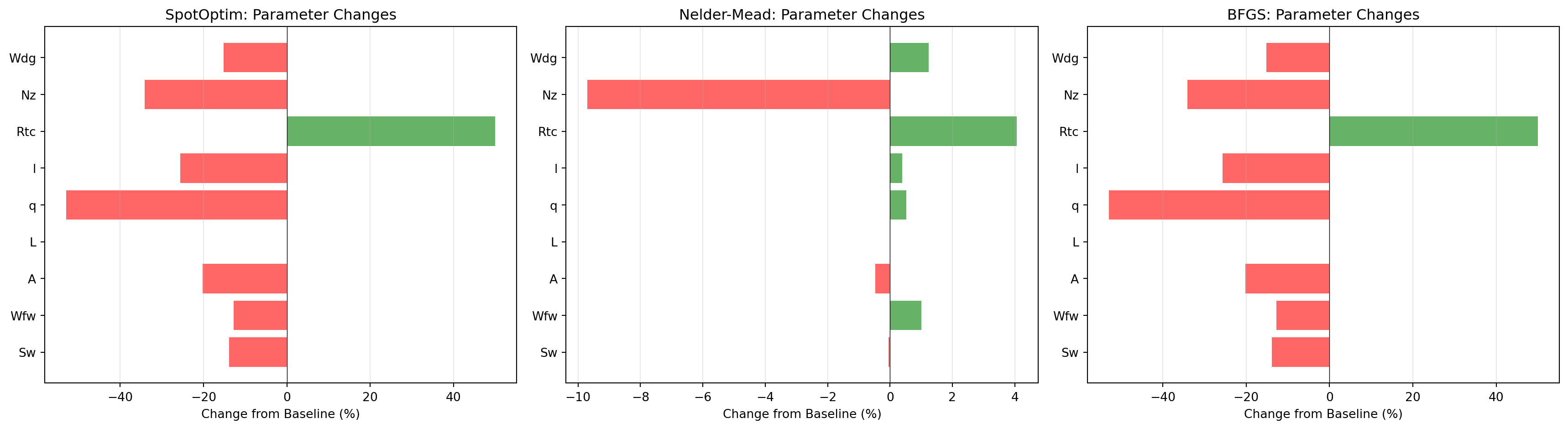
4.16 Key Insights from Optimal Solutions
# Find parameters with largest changes for each method
def analyze_changes(decoded, baseline_decoded, method_name):
    changes = {param_names[i]: decoded[i] - baseline_decoded[i]
               for i in range(len(param_names))}
    sorted_changes = sorted(changes.items(), key=lambda x: abs(x[1]), reverse=True)

    print(f"\n{method_name} - Top 5 Parameter Changes:")
    print("-" * 50)
    for param, change in sorted_changes[:5]:
        idx = param_names.index(param)
        pct = change / baseline_decoded[idx] * 100
        print(f"  {param:5s}: {change:+8.2f} ({pct:+6.1f}%)")

analyze_changes(spot_decoded, baseline_decoded, "SpotOptim")
analyze_changes(nm_decoded, baseline_decoded, "Nelder-Mead")
analyze_changes(bfgs_decoded, baseline_decoded, "BFGS")
SpotOptim - Top 5 Parameter Changes:
--------------------------------------------------
  Wdg  :  -304.00 ( -15.2%)
  Wfw  :   -32.00 ( -12.7%)
  Sw   :   -24.00 ( -13.8%)
  q    :   -17.98 ( -52.9%)
  A    :    -1.52 ( -20.2%)

Nelder-Mead - Top 5 Parameter Changes:
--------------------------------------------------
  Wdg  :   +24.94 (  +1.2%)
  Wfw  :    +2.53 (  +1.0%)
  Nz   :    -0.37 (  -9.7%)
  q    :    +0.18 (  +0.5%)
  L    :    -0.13 (  -inf%)

BFGS - Top 5 Parameter Changes:
--------------------------------------------------
  Wdg  :  -304.00 ( -15.2%)
  Wfw  :   -32.00 ( -12.7%)
  Sw   :   -24.00 ( -13.8%)
  q    :   -17.98 ( -52.9%)
  A    :    -1.52 ( -20.2%)
4.17 Method Efficiency Comparison
# Calculate efficiency metrics
efficiency = pd.DataFrame({
    'Method': ['SpotOptim', 'Nelder-Mead', 'BFGS'],
    'Weight Reduction (lb)': [
        baseline_weight - result_spot.fun,
        baseline_weight - result_nm.fun,
        baseline_weight - result_bfgs.fun
    ],
    'Evals to Best': [
        np.argmin(optimizer_spot.y_) + 1,
        result_nm.nfev,
        result_bfgs.nfev
    ],
    'Time per Eval (ms)': [
        spot_time / result_spot.nfev * 1000,
        nm_time / result_nm.nfev * 1000,
        bfgs_time / result_bfgs.nfev * 1000
    ]
})

print("\n" + "=" * 80)
print("METHOD EFFICIENCY METRICS")
print("=" * 80)
print(efficiency.to_string(index=False))
print("=" * 80)
================================================================================
METHOD EFFICIENCY METRICS
================================================================================
     Method  Weight Reduction (lb)  Evals to Best  Time per Eval (ms)
  SpotOptim             114.404734             25          233.969863
Nelder-Mead              13.363478             30            0.025098
       BFGS             114.404734             60            0.022503
================================================================================
4.18 Visualization: 2D Slices of Optimal Solutions
Let’s visualize how the optimal solutions compare in the most important 2D subspaces:
# Create 2D slices showing optimal points
fig, axes = plt.subplots(2, 2, figsize=(14, 12))

# Important parameter pairs based on sensitivity analysis
pairs = [
    (7, 2),  # Nz vs A (load factor vs aspect ratio)
    (0, 8),  # Sw vs Wdg (wing area vs gross weight)
    (7, 0),  # Nz vs Sw (load factor vs wing area)
    (2, 6)   # A vs Rtc (aspect ratio vs thickness ratio)
]

for ax, (i, j) in zip(axes.flat, pairs):
    # Create meshgrid for contour plot
    x_range = np.linspace(0, 1, 50)
    y_range = np.linspace(0, 1, 50)
    X, Y = np.meshgrid(x_range, y_range)

    # Evaluate function on grid (fixing other parameters at baseline)
    Z = np.zeros_like(X)
    for ii in range(X.shape[0]):
        for jj in range(X.shape[1]):
            point = baseline_coded.copy()
            point[i] = X[ii, jj]
            point[j] = Y[ii, jj]
            Z[ii, jj] = wingwt(point)[0]

    # Plot contours
    contour = ax.contourf(X, Y, Z, levels=20, cmap='viridis', alpha=0.6)
    ax.contour(X, Y, Z, levels=10, colors='black', alpha=0.3, linewidths=0.5)

    # Plot optimal points
    ax.plot(baseline_coded[i], baseline_coded[j], 'go', markersize=12,
            label='Baseline', markeredgecolor='black', markeredgewidth=1.5)
    ax.plot(result_spot.x[i], result_spot.x[j], 'r*', markersize=15,
            label='SpotOptim', markeredgecolor='black', markeredgewidth=1)
    ax.plot(result_nm.x[i], result_nm.x[j], 'bs', markersize=10,
            label='Nelder-Mead', markeredgecolor='black', markeredgewidth=1)
    ax.plot(result_bfgs.x[i], result_bfgs.x[j], 'c^', markersize=10,
            label='BFGS', markeredgecolor='black', markeredgewidth=1)

    ax.set_xlabel(param_names[i])
    ax.set_ylabel(param_names[j])
    ax.set_title(f'{param_names[j]} vs {param_names[i]}')
    ax.legend(loc='best', fontsize=8)
    ax.grid(True, alpha=0.3)

    # Add colorbar
    plt.colorbar(contour, ax=ax, label='Wing Weight (lb)')

plt.tight_layout()
plt.show()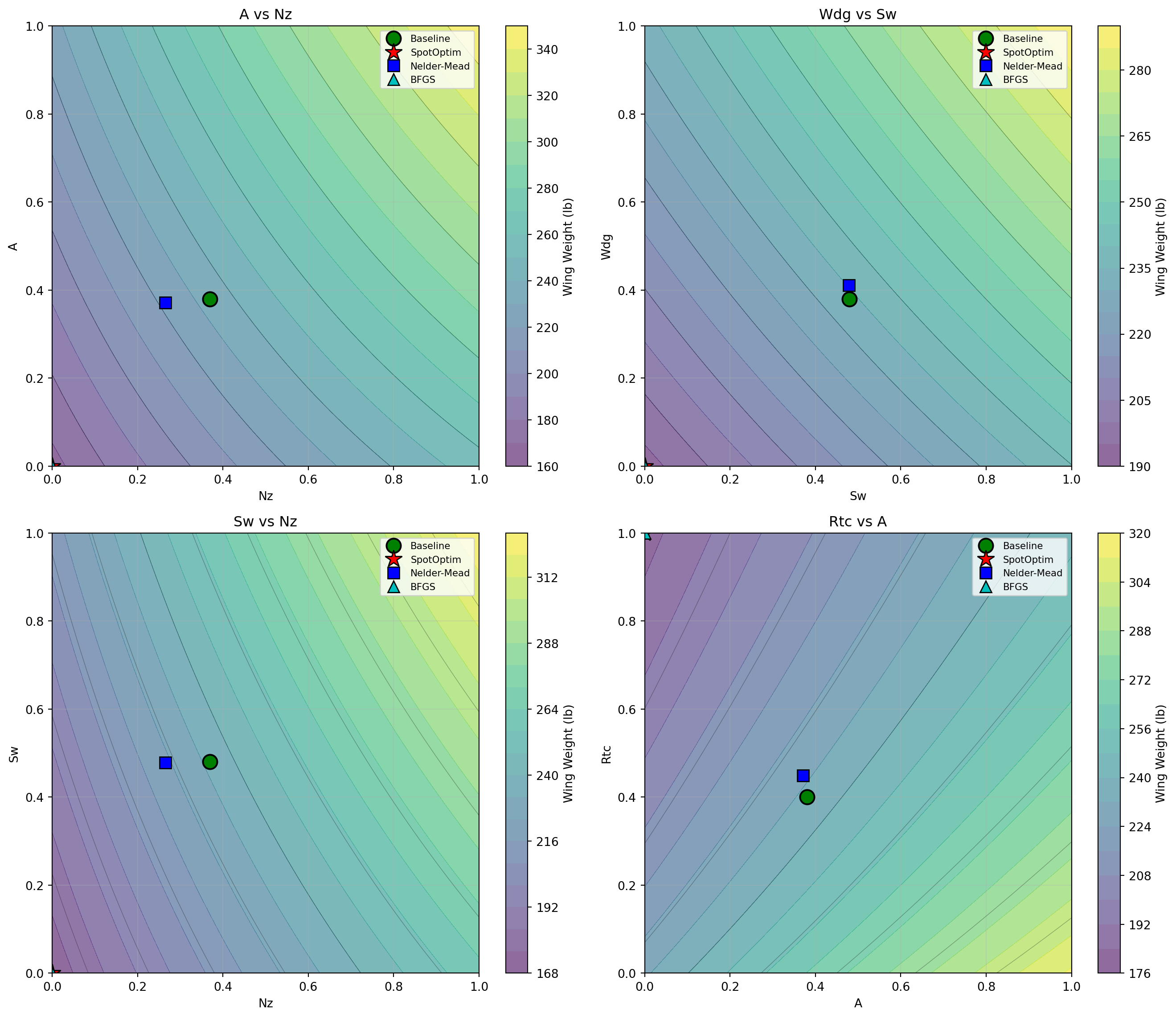
4.19 Conclusion
This analysis demonstrates the application of different optimization methods to the Aircraft Wing Weight Example. Key takeaways:
- SpotOptim provides efficient global optimization with good exploration of the design space
- Nelder-Mead offers robust derivative-free optimization but may require more evaluations
- BFGS converges quickly for smooth problems but can get trapped in local minima
For aircraft design problems with expensive simulations, Bayesian optimization (SpotOptim) offers the best balance of efficiency and solution quality, making it particularly suitable for real-world engineering applications.
4.20 Jupyter Notebook
Note
- The Jupyter-Notebook of this chapter is available on GitHub in the Sequential Parameter Optimization Cookbook Repository