import matplotlib.pyplot as plt
import numpy as np
import torch
import torch.nn as nn
from typing import Tuple
from spotoptim import SpotOptim
from spotoptim.nn.linear_regressor import LinearRegressor28 Hyperparameter Tuning for Physics-Informed Neural Networks
Using SpotOptim to Optimize PINN Architecture and Training
29 Overview
This tutorial demonstrates how to use SpotOptim for hyperparameter optimization of Physics-Informed Neural Networks (PINNs). We’ll optimize the network architecture and training parameters to find the best configuration for solving an ordinary differential equation.
Building on the basic PINN demo, we’ll now systematically search for optimal:
- Number of neurons per hidden layer
- Number of hidden layers
- Activation function (categorical)
- Optimizer algorithm (categorical)
- Learning rate (log-scale)
- Physics loss weight (log-scale)
29.1 Key Features
29.1.1 1. PyTorch Dataset and DataLoader
Following PyTorch best practices from the official tutorial, this tutorial implements:
- Custom Dataset Classes: Separate classes for supervised data (
PINNDataset) and collocation points (CollocationDataset) - DataLoader Integration: Efficient batch processing with configurable batch size, shuffling, and parallel loading
- Proper Data Separation: Clean separation of training, validation, and collocation data
- Gradient Tracking: Automatic gradient handling for collocation points needed in physics loss
Benefits:
- Modularity: Clean separation between data and model code
- Efficiency: Batch processing and optional parallel data loading
- Scalability: Easy to extend to larger datasets
- Best Practices: Follows PyTorch conventions used across the ecosystem
29.1.2 2. Automatic Transformation Handling
This tutorial also showcases SpotOptim’s var_trans feature for automatic variable transformations. Learning rates and regularization parameters are often best explored on a log scale, but manually transforming values is tedious and error-prone. With var_trans, you simply specify:
var_trans = [None, None, "log10", "log10"]SpotOptim then:
- Optimizes internally in log-transformed space (efficient exploration)
- Passes original-scale values to your objective function (no manual conversion needed)
- Displays all results in original scale (easy interpretation)
This eliminates the need for manual 10**x conversions throughout your code!
30 The Problem
We’re solving the same ODE as in the basic PINN demo:
\[ \frac{dy}{dt} + 0.1 y - \sin\left(\frac{\pi t}{2}\right) = 0 \]
with initial condition \(y(0) = 0\).
31 Setup
# Set random seed for reproducibility
torch.manual_seed(42)
np.random.seed(42)
Set number of epochs for training, maximum number of iterations for hyperparameter optimization, and initial design size. For this example we use a small number of epochs and iterations to keep the runtime short.
N_EPOCHS = 500
MAX_ITER = 15
N_INITIAL = 10
32 Data Generation
Following PyTorch best practices, we’ll create custom Dataset classes for our PINN data.
32.1 Custom Dataset Classes
We’ll create two dataset types:
PINNDatasetfor supervised data (training and validation)CollocationDatasetfor physics-informed collocation points
from torch.utils.data import Dataset, DataLoader

def oscillator(
    n_steps: int = 3000,
    t_min: float = 0.0,
    t_max: float = 30.0,
    y0: float = 0.0,
    alpha: float = 0.1,
    omega: float = np.pi / 2
) -> Tuple[torch.Tensor, torch.Tensor]:
    """
    Solve ODE: dy/dt + alpha*y - sin(omega*t) = 0
    using RK2 (midpoint method).

    Returns:
        t_tensor: Time points, shape (n_steps, 1)
        y_tensor: Solution values, shape (n_steps, 1)
    """
    t_step = (t_max - t_min) / n_steps
    t_points = np.arange(t_min, t_min + n_steps * t_step, t_step)[:n_steps]

    y = [y0]

    for t_current_step_end in t_points[1:]:
        t_midpoint = t_current_step_end - t_step / 2.0
        y_prev = y[-1]

        slope_at_t_mid = -alpha * y_prev + np.sin(omega * t_midpoint)
        y_intermediate = y_prev + (t_step / 2.0) * slope_at_t_mid

        slope_at_t_end = -alpha * y_intermediate + np.sin(omega * t_current_step_end)
        y_next = y_prev + t_step * slope_at_t_end
        y.append(y_next)

    t_tensor = torch.tensor(t_points, dtype=torch.float32).view(-1, 1)
    y_tensor = torch.tensor(y, dtype=torch.float32).view(-1, 1)

    return t_tensor, y_tensor
class PINNDataset(Dataset):
"""PyTorch Dataset for PINN supervised data (training/validation).
This dataset stores time-solution pairs (t, y) for supervised learning.
Args:
t (torch.Tensor): Time points, shape (n_samples, 1)
y (torch.Tensor): Solution values, shape (n_samples, 1)
"""
def __init__(self, t: torch.Tensor, y: torch.Tensor):
self.t = t
self.y = y
def __len__(self) -> int:
return len(self.t)
def __getitem__(self, idx: int) -> Tuple[torch.Tensor, torch.Tensor]:
return self.t[idx], self.y[idx]class CollocationDataset(Dataset):
"""PyTorch Dataset for PINN collocation points.
This dataset stores time points where physics loss is evaluated.
Gradients are required for computing derivatives in the PDE.
Args:
t (torch.Tensor): Collocation time points, shape (n_points, 1)
"""
def __init__(self, t: torch.Tensor):
# Store collocation points with gradient tracking
self.t = t.requires_grad_(True)
def __len__(self) -> int:
return len(self.t)
def __getitem__(self, idx: int) -> torch.Tensor:
# Return single collocation point (still requires_grad)
return self.t[idx].unsqueeze(0)Generate exact solution using Runge-Kutta 2 (RK2) method:
x_exact, y_exact = oscillator()

# Create training data (sparse sampling)
t_train = x_exact[0:3000:119]
y_train = y_exact[0:3000:119]

# Create validation data (different sampling for unbiased evaluation)
t_val = x_exact[50:3000:120]
y_val = y_exact[50:3000:120]

# Create collocation points for physics loss
t_physics = torch.linspace(0, 30, 50).view(-1, 1)

# Create Dataset objects
train_dataset = PINNDataset(t_train, y_train)
val_dataset = PINNDataset(t_val, y_val)
collocation_dataset = CollocationDataset(t_physics)

print(f"Training dataset size: {len(train_dataset)}")
print(f"Validation dataset size: {len(val_dataset)}")
print(f"Collocation dataset size: {len(collocation_dataset)}")
print(f"\nSample from training dataset:")
t_sample, y_sample = train_dataset[0]
print(f"  t: {t_sample.item():.4f}, y: {y_sample.item():.4f}")
Training dataset size: 26
Validation dataset size: 25
Collocation dataset size: 50
Sample from training dataset:
t: 0.0000, y: 0.000033 Define the PINN Training Function
This function creates DataLoaders and trains a PINN with given hyperparameters. Following PyTorch best practices, we use DataLoader for efficient batch processing.
def train_pinn(
    l1: int,
    num_layers: int,
    activation: str,
    optimizer_name: str,
    lr_unified: float,
    alpha: float,
    n_epochs: int = N_EPOCHS,
    batch_size: int = 16,
    verbose: bool = False
) -> float:
    """
    Train a PINN with specified hyperparameters using DataLoaders.

    Args:
        l1: Number of neurons per hidden layer
        num_layers: Number of hidden layers
        activation: Activation function ("Tanh", "ReLU", "Sigmoid", "GELU")
        optimizer_name: Optimizer algorithm ("Adam", "SGD", "RMSprop", "AdamW")
        lr_unified: Unified learning rate multiplier
        alpha: Weight for physics loss
        n_epochs: Number of training epochs
        batch_size: Batch size for DataLoader
        verbose: Whether to print progress

    Returns:
        Validation mean squared error
    """
    # Set seed for reproducibility
    torch.manual_seed(42)

    # Create DataLoaders
    train_loader = DataLoader(
        train_dataset,
        batch_size=batch_size,
        shuffle=True,
        num_workers=0,
        pin_memory=False
    )

    val_loader = DataLoader(
        val_dataset,
        batch_size=batch_size,
        shuffle=False,
        num_workers=0,
        pin_memory=False
    )

    # For collocation points, we can use full batch since it's small
    collocation_loader = DataLoader(
        collocation_dataset,
        batch_size=len(collocation_dataset),
        shuffle=False,
        num_workers=0
    )

    # Create model
    model = LinearRegressor(
        input_dim=1,
        output_dim=1,
        l1=l1,
        num_hidden_layers=num_layers,
        activation=activation,
        lr=lr_unified
    )

    # Get optimizer
    optimizer = model.get_optimizer(optimizer_name)

    # Training loop
    for epoch in range(n_epochs):
        model.train()
        epoch_loss = 0.0

        # Get collocation points (full batch)
        t_physics_batch = next(iter(collocation_loader))
        # Ensure gradients are enabled
        t_physics_batch = t_physics_batch.requires_grad_(True)

        # Iterate over training batches
        for batch_t, batch_y in train_loader:
            optimizer.zero_grad()

            # Data Loss
            y_pred = model(batch_t)
            loss_data = torch.mean((y_pred - batch_y)**2)

            # Physics Loss (computed on full collocation set)
            y_physics = model(t_physics_batch)
            dy_dt = torch.autograd.grad(
                y_physics,
                t_physics_batch,
                torch.ones_like(y_physics),
                create_graph=True,
                retain_graph=True
            )[0]

            # PDE residual: dy/dt + 0.1*y - sin(pi*t/2) = 0
            physics_residual = dy_dt + 0.1 * y_physics - torch.sin(np.pi * t_physics_batch / 2)
            loss_physics = torch.mean(physics_residual**2)

            # Total Loss
            loss = loss_data + alpha * loss_physics
            loss.backward()
            optimizer.step()

            epoch_loss += loss.item()

        if verbose and (epoch + 1) % 2000 == 0:
            avg_loss = epoch_loss / len(train_loader)
            print(f"  Epoch {epoch+1}/{n_epochs}: Avg Loss = {avg_loss:.6f}")

    # Evaluate on validation set
    model.eval()
    val_mse = 0.0
    with torch.no_grad():
        for batch_t, batch_y in val_loader:
            y_pred = model(batch_t)
            val_mse += torch.mean((batch_y - y_pred)**2).item()

    val_mse /= len(val_loader)
    return val_mse

# Test the function with default parameters
print("Testing PINN training function with DataLoaders...")
test_error = train_pinn(
    l1=32,
    num_layers=2,
    activation="Tanh",
    optimizer_name="Adam",
    lr_unified=3.0,
    alpha=0.06,
    batch_size=16,
    n_epochs=N_EPOCHS,
    verbose=True
)
print(f"\nTest validation MSE: {test_error:.6f}")
Testing PINN training function with DataLoaders...
Test validation MSE: 0.18875234 Hyperparameter Optimization with SpotOptim
Now we’ll use SpotOptim to find the best hyperparameters:
34.1 Define the Objective Function
def objective_pinn(X):
    """
    Objective function for SpotOptim.

    Args:
        X: Array of hyperparameter configurations, shape (n_configs, 6)
           Each row: [l1, num_layers, activation, optimizer, lr_unified, alpha]
           Note: SpotOptim handles log transformations and factor mapping automatically

    Returns:
        Array of validation errors
    """
    results = []

    for i, params in enumerate(X):
        # Extract parameters (already in original scale thanks to var_trans)
        # Factor variables (activation, optimizer) are returned as strings
        l1 = int(params[0])                    # Number of neurons
        num_layers = int(params[1])            # Number of hidden layers
        activation = params[2]                 # Activation function
        optimizer_name = params[3]             # Optimizer algorithm
        lr_unified = params[4]                 # Learning rate
        alpha = params[5]                      # Physics weight

        print(f"\nConfiguration {i+1}/{len(X)}:")
        print(f"  l1={l1}, num_layers={num_layers}, activation={activation}, ")
        print(f"  optimizer={optimizer_name}, lr_unified={lr_unified:.4f}, alpha={alpha:.4f}")

        # Train PINN with these hyperparameters
        val_error = train_pinn(
            l1=l1,
            num_layers=num_layers,
            activation=activation,
            optimizer_name=optimizer_name,
            lr_unified=lr_unified,
            alpha=alpha,
            n_epochs=N_EPOCHS,
            verbose=False
        )

        print(f"  Validation MSE: {val_error:.6f}")
        results.append(val_error)

    return np.array(results)
We test the objective function with two configurations:
X_test = np.array([
    [32, 2, "Tanh", "Adam", 3.0, 0.06],    # Baseline config
    [64, 3, "ReLU", "AdamW", 2.0, 0.04]    # Alternative config
], dtype=object)
test_results = objective_pinn(X_test)
print(f"\nTest results: {test_results}")
Configuration 1/2:
  l1=32, num_layers=2, activation=Tanh,
  optimizer=Adam, lr_unified=3.0000, alpha=0.0600
  Validation MSE: 0.188752

Configuration 2/2:
  l1=64, num_layers=3, activation=ReLU,
  optimizer=AdamW, lr_unified=2.0000, alpha=0.0400
  Validation MSE: 0.168650

Test results: [0.18875157 0.16864995]
34.2 Run the Optimization
Use tensorboard --logdir=runs from a shell in the current directory (where this notebook is located) to visualize the optimization process.
Setting the bounds for the search space:
# Define search space with var_trans for automatic log-scale handling
bounds = [
    (16, 128),                                      # l1: neurons per layer (16 to 128)
    (1, 4),                                         # num_layers: 1 to 4 hidden layers
    ("Tanh", "ReLU", "Sigmoid", "GELU"),         # activation: activation function
    ("Adam", "SGD", "RMSprop", "AdamW"),          # optimizer: optimizer algorithm
    (0.1, 10.0),                                    # lr_unified: learning rate (0.1 to 10)
    (0.01, 1.0)                                     # alpha: physics weight (0.01 to 1.0)
]
Specify the variable types and transformations. Use var_trans to handle log-scale transformations automatically, factor variables don’t need transformations (None):
var_type = ["int", "int", "factor", "factor", "float", "float"]
var_name = ["l1", "num_layers", "activation", "optimizer", "lr_unified", "alpha"]
var_trans = [None, None, None, None, "log10", "log10"]
# Create optimizer
optimizer = SpotOptim(
fun=objective_pinn,
bounds=bounds,
var_type=var_type,
var_name=var_name,
var_trans=var_trans, # Automatic log-scale handling!
max_iter=MAX_ITER,
n_initial=N_INITIAL,
seed=42,
verbose=True,
tensorboard_clean=True,
tensorboard_log=True
)Factor variable at dimension 2:
Levels: ['Tanh', 'ReLU', 'Sigmoid', 'GELU']
Mapped to integers: 0 to 3
Factor variable at dimension 3:
Levels: ['Adam', 'SGD', 'RMSprop', 'AdamW']
Mapped to integers: 0 to 3
Removed old TensorBoard logs: runs/spotoptim_20260701_204423
Cleaned 1 old TensorBoard log directory
TensorBoard logging enabled: runs/spotoptim_20260701_211045/var/folders/dw/pvtj6mt91znd0hftcztqb0k00000gn/T/ipykernel_40425/2553769193.py:2: UserWarning: Factor variables detected (original bounds dimensions: [2, 3]) but the active surrogate (GaussianProcessRegressor) does not support nominal (order-agnostic) factor metrics. Factor integer codes will be treated as ordinal numbers, which may mislead the surrogate. Consider using a factor-aware Kriging surrogate: Kriging(metric_factorial='hamming').
optimizer = SpotOptim(Display search space configuration. The transcolumn shows applied transformations. lr_unified and alpha use log10 transformation internally. This enables efficient exploration of log-scale parameters. All values shown are in original scale (not transformed).
design_table = optimizer.get_design_table(tablefmt="github")
print(design_table)
| name | type | lower | upper | default | transform |
|------------|--------|---------|----------|-----------|-------------|
| l1 | int | 16.0000 | 128.0000 | 72 | - |
| num_layers | int | 1.0000 | 4.0000 | 2 | - |
| activation | factor | - | - | Sigmoid | - |
| optimizer | factor | - | - | RMSprop | - |
| lr_unified | float | 0.1000 | 10.0000 | 5.0500 | log10 |
| alpha | float | 0.0100 | 1.0000 | 0.5050 | log10 |Run optimization
result = optimizer.optimize()
Configuration 1/10:
  l1=28, num_layers=2, activation=Sigmoid,
  optimizer=RMSprop, lr_unified=1.0211, alpha=0.0923
  Validation MSE: 0.192541

Configuration 2/10:
  l1=117, num_layers=3, activation=ReLU,
  optimizer=SGD, lr_unified=0.4832, alpha=0.0146
  Validation MSE: 0.205611

Configuration 3/10:
  l1=92, num_layers=1, activation=Tanh,
  optimizer=SGD, lr_unified=6.5194, alpha=0.6267
  Validation MSE: nan

Configuration 4/10:
  l1=41, num_layers=4, activation=ReLU,
  optimizer=Adam, lr_unified=0.2742, alpha=0.1697
  Validation MSE: 0.185978

Configuration 5/10:
  l1=105, num_layers=2, activation=ReLU,
  optimizer=AdamW, lr_unified=0.1136, alpha=0.0176
  Validation MSE: 0.202467

Configuration 6/10:
  l1=24, num_layers=1, activation=Sigmoid,
  optimizer=RMSprop, lr_unified=4.4408, alpha=0.0293
  Validation MSE: 0.189705

Configuration 7/10:
  l1=83, num_layers=3, activation=GELU,
  optimizer=AdamW, lr_unified=0.2277, alpha=0.2652
  Validation MSE: 0.181881

Configuration 8/10:
  l1=65, num_layers=2, activation=Tanh,
  optimizer=SGD, lr_unified=3.4389, alpha=0.9830
  Validation MSE: 0.195487

Configuration 9/10:
  l1=116, num_layers=3, activation=Sigmoid,
  optimizer=RMSprop, lr_unified=0.8521, alpha=0.1020
  Validation MSE: 0.180443

Configuration 10/10:
  l1=51, num_layers=4, activation=Sigmoid,
  optimizer=Adam, lr_unified=1.6729, alpha=0.0458
  Validation MSE: 0.205772
Warning: 1 initial design point(s) returned NaN/inf and will be ignored (reduced from 10 to 9 points)
Note: Initial design size (9) is smaller than requested (10) due to NaN/inf values
Initial best: f(x) = 0.180443

Configuration 1/1:
  l1=100, num_layers=2, activation=Sigmoid,
  optimizer=RMSprop, lr_unified=0.1469, alpha=0.0131
  Validation MSE: 0.196912
Iter 1 | Best: 0.180443 | Curr: 0.196912 | Rate: 0.00 | Evals: 66.7%

Configuration 1/1:
  l1=94, num_layers=1, activation=Sigmoid,
  optimizer=SGD, lr_unified=3.6048, alpha=0.0374
  Validation MSE: 0.196974
Iter 2 | Best: 0.180443 | Curr: 0.196974 | Rate: 0.00 | Evals: 73.3%

Configuration 1/1:
  l1=96, num_layers=3, activation=GELU,
  optimizer=RMSprop, lr_unified=0.2996, alpha=0.1593
  Validation MSE: 0.169332
Iter 3 | Best: 0.169332 | Rate: 0.33 | Evals: 80.0%

Configuration 1/1:
  l1=127, num_layers=1, activation=Sigmoid,
  optimizer=SGD, lr_unified=1.9791, alpha=0.2477
  Validation MSE: 0.208434
Iter 4 | Best: 0.169332 | Curr: 0.208434 | Rate: 0.25 | Evals: 86.7%

Configuration 1/1:
  l1=78, num_layers=3, activation=Sigmoid,
  optimizer=SGD, lr_unified=0.5950, alpha=0.4743
  Validation MSE: 0.228979
Iter 5 | Best: 0.169332 | Curr: 0.228979 | Rate: 0.20 | Evals: 93.3%

Configuration 1/1:
  l1=81, num_layers=2, activation=Sigmoid,
  optimizer=Adam, lr_unified=0.2781, alpha=0.0168
  Validation MSE: 0.202393
Iter 6 | Best: 0.169332 | Curr: 0.202393 | Rate: 0.17 | Evals: 100.0%
TensorBoard writer closed. View logs with: tensorboard --logdir=runs/spotoptim_20260701_211045
35 Results Analysis
35.1 Best Configuration
Display best hyperparameters using print_best() method. With var_trans, results are already in original scale!
optimizer.print_best(result)
Best Solution Found:
--------------------------------------------------
  l1: 96
  num_layers: 3
  activation: GELU
  optimizer: RMSprop
  lr_unified: 0.2996
  alpha: 0.1593
  Objective Value: 0.1693
  Total Evaluations: 15
Store values for later use in visualizations. Values are already in original scale thanks to var_trans. Factor variables are returned as strings.
best_l1 = int(result.x[0])
best_num_layers = int(result.x[1])
best_activation = result.x[2]
best_optimizer = result.x[3]
best_lr_unified = result.x[4]
best_alpha = result.x[5]
best_val_error = result.fun

print(f"Best activation: {best_activation}")
print(f"Best optimizer: {best_optimizer}")
Best activation: GELU
Best optimizer: RMSprop35.1.1 Results Table with Importance Scores
Display comprehensive results table with importance scores
table = optimizer.get_results_table(show_importance=True, tablefmt="github")
print(table)
| name | type | default | lower | upper | tuned | transform | importance | stars |
|------------|--------|-----------|---------|----------|---------|-------------|--------------|---------|
| l1 | int | 72 | 16.0000 | 128.0000 | 96 | - | 10.2 | . |
| num_layers | int | 2 | 1.0000 | 4.0000 | 3 | - | 10.96 | . |
| activation | factor | Sigmoid | - | - | GELU | - | 28 | . |
| optimizer | factor | RMSprop | - | - | RMSprop | - | 35.84 | . |
| lr_unified | float | 5.0500 | 0.1000 | 10.0000 | 0.2996 | log10 | 2.39 | |
| alpha | float | 0.5050 | 0.0100 | 1.0000 | 0.1593 | log10 | 12.62 | . |
Interpretation: ***: >99%, **: >75%, *: >50%, .: >10%35.2 Optimization History
optimizer.plot_progress(log_y=True, ylabel="Validation MSE")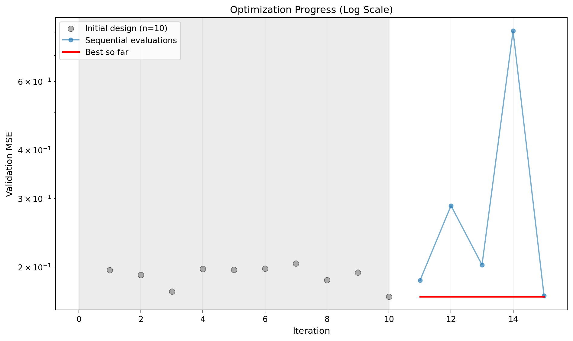
35.3 Surrogate Visualization
Visualize the surrogate model’s learned response surface for the most important hyperparameter combinations:
# Plot top 3 most important hyperparameter combinations
optimizer.plot_important_hyperparameter_contour(max_imp=3)
Plotting surrogate contours for top 3 most important parameters:
optimizer: importance = 35.84% (type: factor)
activation: importance = 28.00% (type: factor)
alpha: importance = 12.62% (type: float)
Generating 3 surrogate plots...
Plotting optimizer vs activation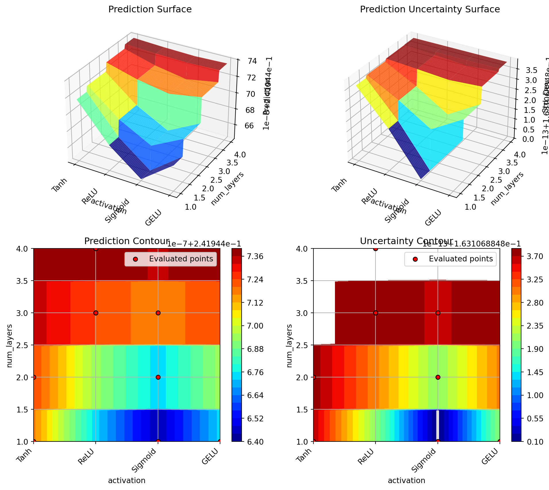
Plotting optimizer vs alpha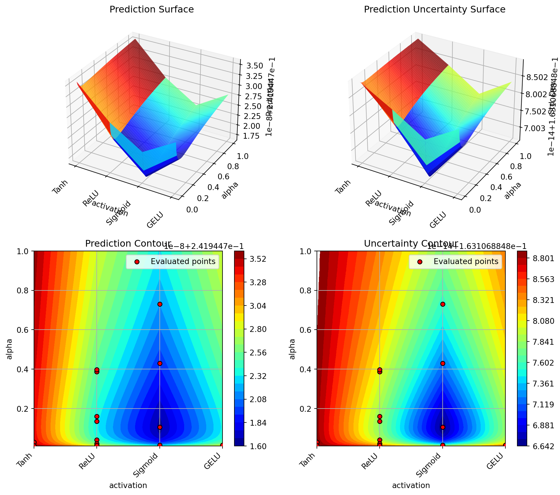
Plotting activation vs alpha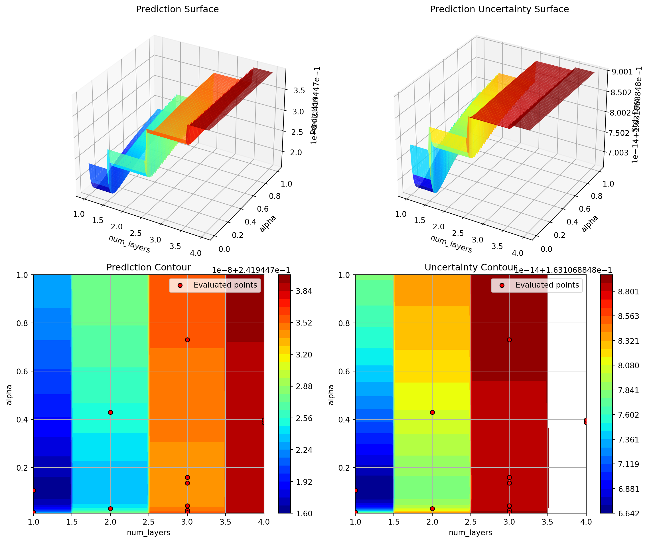
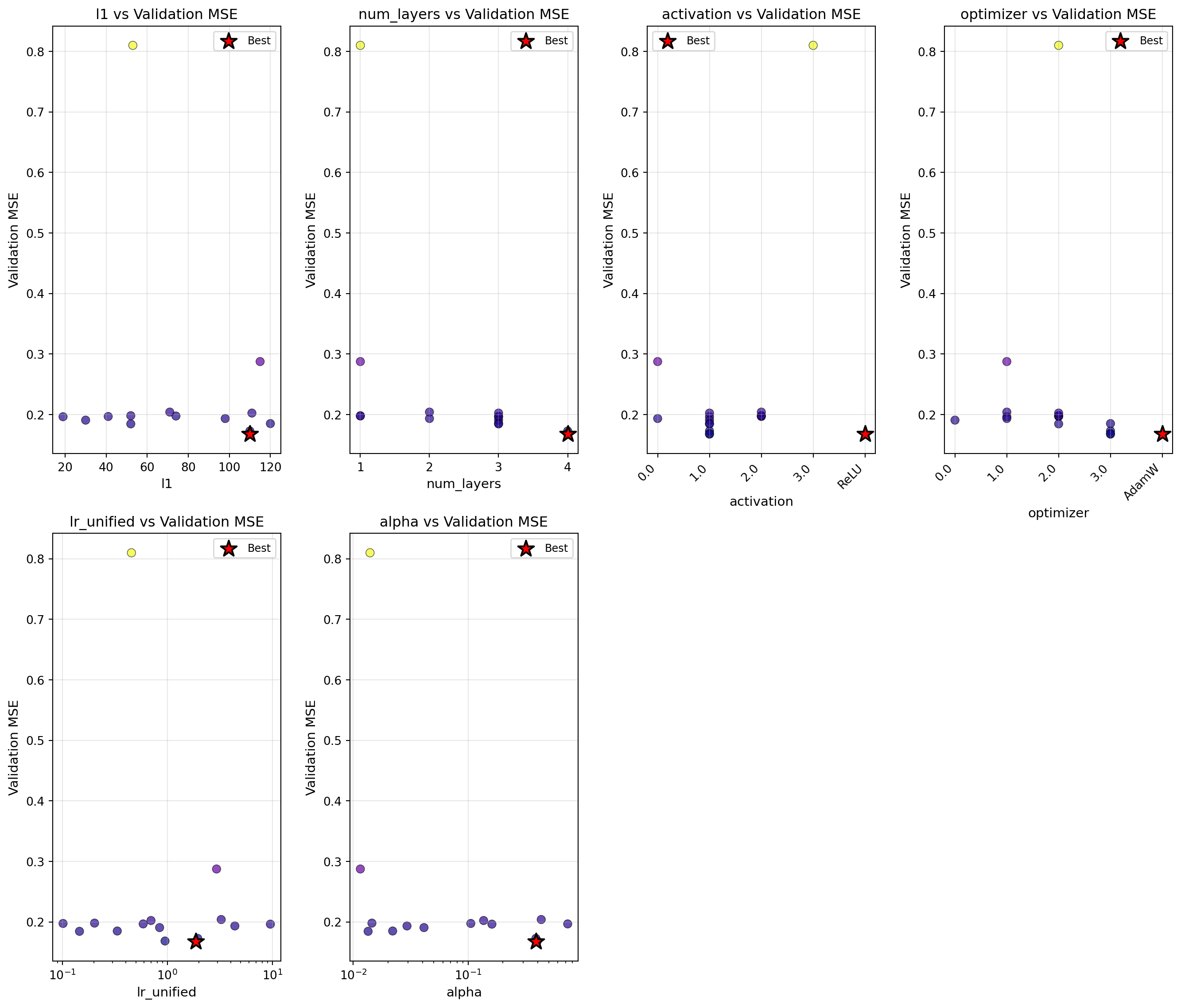
35.4 Parameter Distribution Analysis
optimizer.plot_parameter_scatter(
    result,
    ylabel="Validation MSE",
    cmap="plasma",
    figsize=(14, 12)
)
36 Train Final Model with Best Hyperparameters
Now let’s train a final model with the optimized hyperparameters using DataLoaders:
print("Training final model with best hyperparameters using DataLoaders...")
print(f"Training for 30,000 epochs...")

# Set seed for reproducibility
torch.manual_seed(42)

# Create DataLoaders for final training
final_batch_size = 16
train_loader_final = DataLoader(
    train_dataset,
    batch_size=final_batch_size,
    shuffle=True,
    num_workers=0
)

collocation_loader_final = DataLoader(
    collocation_dataset,
    batch_size=len(collocation_dataset),
    shuffle=False,
    num_workers=0
)

# Create model with best hyperparameters
final_model = LinearRegressor(
    input_dim=1,
    output_dim=1,
    l1=best_l1,
    num_hidden_layers=best_num_layers,
    activation=best_activation,
    lr=best_lr_unified
)

optimizer_final = final_model.get_optimizer(best_optimizer)

# Training with history tracking
loss_history = []
n_epochs_final = 30000

for epoch in range(n_epochs_final):
    final_model.train()
    epoch_loss = 0.0

    # Get collocation points
    t_physics_batch = next(iter(collocation_loader_final))
    t_physics_batch = t_physics_batch.requires_grad_(True)

    # Iterate over training batches
    for batch_t, batch_y in train_loader_final:
        optimizer_final.zero_grad()

        # Data Loss
        y_pred = final_model(batch_t)
        loss_data = torch.mean((y_pred - batch_y)**2)

        # Physics Loss
        y_physics = final_model(t_physics_batch)
        dy_dt = torch.autograd.grad(
            y_physics,
            t_physics_batch,
            torch.ones_like(y_physics),
            create_graph=True,
            retain_graph=True
        )[0]

        physics_residual = dy_dt + 0.1 * y_physics - torch.sin(np.pi * t_physics_batch / 2)
        loss_physics = torch.mean(physics_residual**2)

        # Total Loss
        loss = loss_data + best_alpha * loss_physics
        loss.backward()
        optimizer_final.step()

        epoch_loss += loss.item()

    # Record average loss every 100 epochs
    if (epoch + 1) % 100 == 0:
        avg_loss = epoch_loss / len(train_loader_final)
        loss_history.append(avg_loss)

    if (epoch + 1) % 5000 == 0:
        avg_loss = epoch_loss / len(train_loader_final)
        print(f"  Epoch {epoch+1}/{n_epochs_final}: Avg Loss = {avg_loss:.6f}")

print("Training completed!")

# Plot training history
plt.figure(figsize=(10, 5))
plt.plot(loss_history, linewidth=1.5)
plt.xlabel('Iteration (×100)', fontsize=11)
plt.ylabel('Average Total Loss per Batch', fontsize=11)
plt.title('Final Model Training History', fontsize=12)
plt.grid(True, alpha=0.3)
plt.yscale('log')
plt.tight_layout()
plt.show()
Training final model with best hyperparameters using DataLoaders...
Training for 30,000 epochs...
Epoch 5000/30000: Avg Loss = 0.182355
Epoch 10000/30000: Avg Loss = 0.143730
Epoch 15000/30000: Avg Loss = 0.133864
Epoch 20000/30000: Avg Loss = 0.126419
Epoch 25000/30000: Avg Loss = 0.084283
Epoch 30000/30000: Avg Loss = 0.002897
Training completed!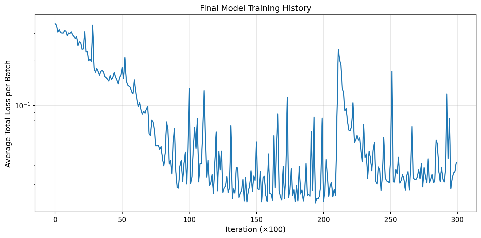
37 Evaluate Final Model
# Create validation DataLoader for evaluation
val_loader_final = DataLoader(
    val_dataset,
    batch_size=len(val_dataset),
    shuffle=False,
    num_workers=0
)

# Evaluate on validation set
final_model.eval()
with torch.no_grad():
    # Validation MSE using DataLoader
    val_mse_total = 0.0
    for batch_t, batch_y in val_loader_final:
        y_pred = final_model(batch_t)
        val_mse_total += torch.mean((y_pred - batch_y)**2).item()
    final_val_mse = val_mse_total / len(val_loader_final)

    # Predict on full domain for visualization
    y_pred_full = final_model(x_exact)
    full_mse = torch.mean((y_pred_full - y_exact)**2).item()

    # Compute maximum absolute error
    max_error = torch.max(torch.abs(y_pred_full - y_exact)).item()

print("\nFinal Model Performance:")
print("-" * 50)
print(f"  Validation MSE: {final_val_mse:.6f}")
print(f"  Full domain MSE: {full_mse:.6f}")
print(f"  Maximum absolute error: {max_error:.6f}")
Final Model Performance:
--------------------------------------------------
  Validation MSE: 0.002740
  Full domain MSE: 0.002078
  Maximum absolute error: 0.119569
38 Visualize Final Solution
# Generate predictions
final_model.eval()
with torch.no_grad():
    y_pred = final_model(x_exact)

fig, axes = plt.subplots(2, 1, figsize=(12, 10))

# Plot 1: Solution comparison
ax1 = axes[0]
ax1.plot(x_exact.numpy(), y_exact.numpy(), 'b-', linewidth=2.5,
         label='Exact solution', alpha=0.8)
ax1.plot(x_exact.numpy(), y_pred.numpy(), 'r--', linewidth=2,
         label='PINN prediction (optimized)', alpha=0.8)

# Plot training data from dataset
ax1.scatter(train_dataset.t.numpy(), train_dataset.y.numpy(),
            color='tab:orange', s=80, label='Training data',
            zorder=5, edgecolors='black', linewidth=0.5)

# Plot collocation points
t_collocation = collocation_dataset.t.detach()
ax1.scatter(t_collocation.numpy(),
            final_model(t_collocation).detach().numpy(),
            color='green', marker='x', s=50,
            label='Collocation points', alpha=0.7, zorder=4)

ax1.set_xlabel('Time t', fontsize=12)
ax1.set_ylabel('Solution y(t)', fontsize=12)
ax1.set_title('Optimized PINN Solution vs Exact Solution', fontsize=13, fontweight='bold')
ax1.legend(fontsize=11, loc='best')
ax1.grid(True, alpha=0.3)

# Plot 2: Error
ax2 = axes[1]
error = torch.abs(y_pred - y_exact)
ax2.plot(x_exact.numpy(), error.numpy(), 'r-', linewidth=2)
ax2.axhline(y=max_error, color='gray', linestyle='--', linewidth=1,
            label=f'Max error = {max_error:.6f}')
ax2.set_xlabel('Time t', fontsize=12)
ax2.set_ylabel('Absolute Error |y_exact - y_PINN|', fontsize=12)
ax2.set_title('Approximation Error (Optimized Model)', fontsize=13, fontweight='bold')
ax2.legend(fontsize=11)
ax2.grid(True, alpha=0.3)

plt.tight_layout()
plt.show()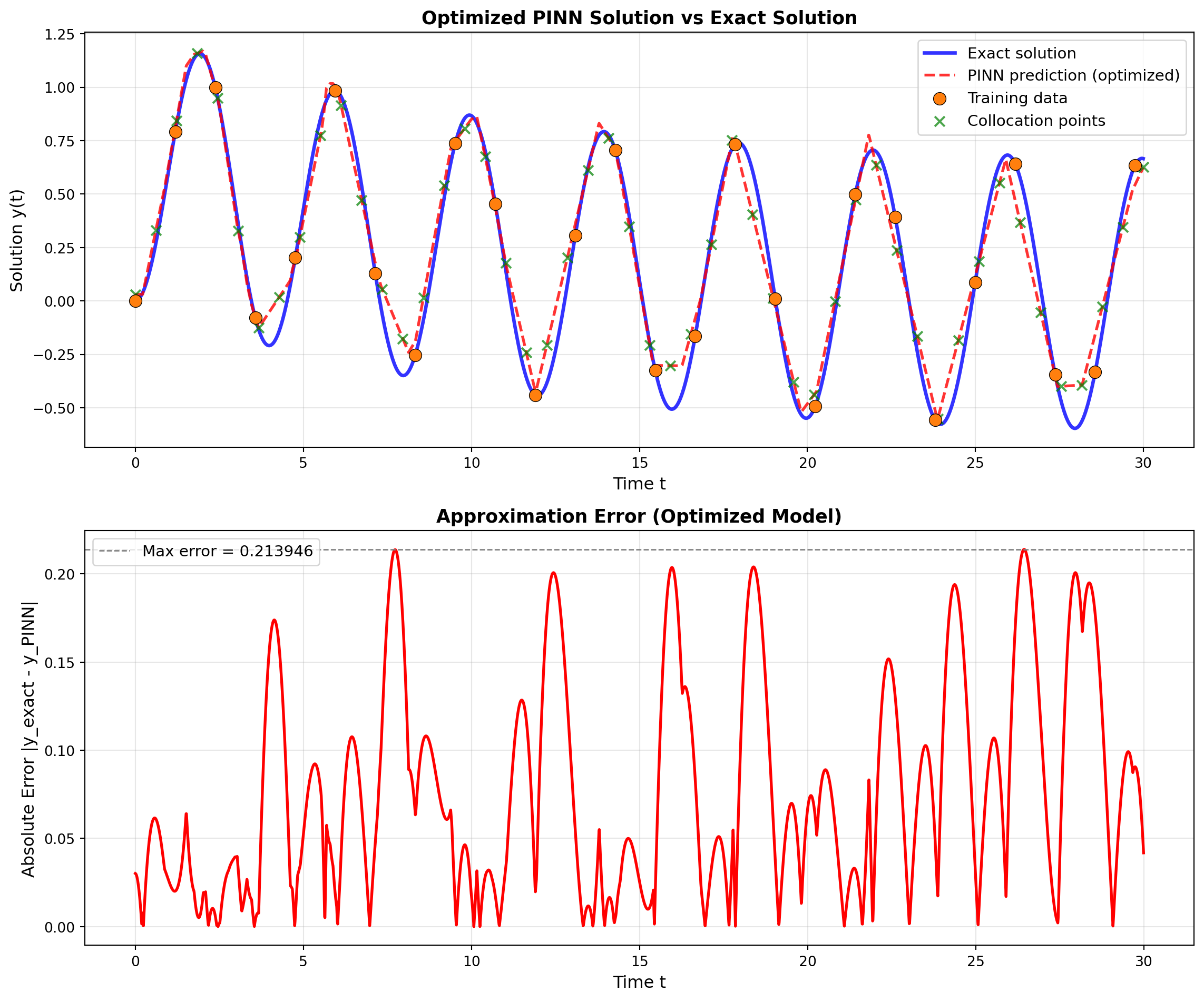
39 Comparison with Baseline
Let’s compare the optimized configuration with a baseline:
print("Training baseline model for comparison...")

# Baseline configuration (from basic PINN demo)
baseline_config = {
    'l1': 32,
    'num_layers': 3,
    'activation': 'Tanh',
    'optimizer': 'Adam',
    'lr_unified': 3.0,
    'alpha': 0.06
}

print(f"\nBaseline Configuration:")
for key, val in baseline_config.items():
    print(f"  {key}: {val}")

# Train baseline
baseline_error = train_pinn(
    l1=baseline_config['l1'],
    num_layers=baseline_config['num_layers'],
    activation=baseline_config['activation'],
    optimizer_name=baseline_config['optimizer'],
    lr_unified=baseline_config['lr_unified'],
    alpha=baseline_config['alpha'],
    n_epochs=N_EPOCHS,
    verbose=False
)

print(f"\nValidation MSE Comparison:")
print("-" * 50)
print(f"  Baseline: {baseline_error:.6f}")
print(f"  Optimized: {best_val_error:.6f}")
print(f"  Improvement: {(1 - best_val_error/baseline_error)*100:.1f}%")

# Bar plot comparison
fig, ax = plt.subplots(figsize=(8, 6))
configs = ['Baseline', 'Optimized']
errors = [baseline_error, best_val_error]
colors = ['tab:blue', 'tab:green']

bars = ax.bar(configs, errors, color=colors, alpha=0.7, edgecolor='black', linewidth=1.5)

# Add value labels on bars
for bar, error in zip(bars, errors):
    height = bar.get_height()
    ax.text(bar.get_x() + bar.get_width()/2., height,
            f'{error:.6f}',
            ha='center', va='bottom', fontsize=11, fontweight='bold')

ax.set_ylabel('Validation MSE', fontsize=12)
ax.set_title('Model Comparison: Baseline vs Optimized', fontsize=13, fontweight='bold')
ax.grid(True, alpha=0.3, axis='y')
plt.tight_layout()
plt.show()
Training baseline model for comparison...
Baseline Configuration:
l1: 32
num_layers: 3
activation: Tanh
optimizer: Adam
lr_unified: 3.0
alpha: 0.06
Validation MSE Comparison:
--------------------------------------------------
Baseline: 0.185787
Optimized: 0.169332
Improvement: 8.9%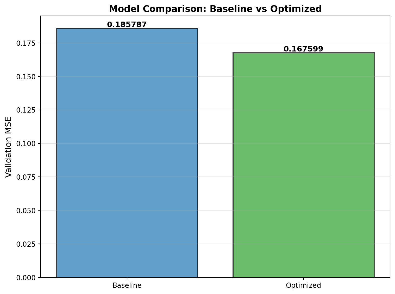
40 Hyperparameter Sensitivity Analysis
Let’s analyze how sensitive the model is to each hyperparameter using the enhanced plot_parameter_scatter() method with Spearman correlation:
# Use the enhanced plot_parameter_scatter method with correlation display
optimizer.plot_parameter_scatter(
    result,
    ylabel="Validation MSE",
    cmap="plasma",
    figsize=(15, 10),
    show_correlation=True,
    log_y=True
)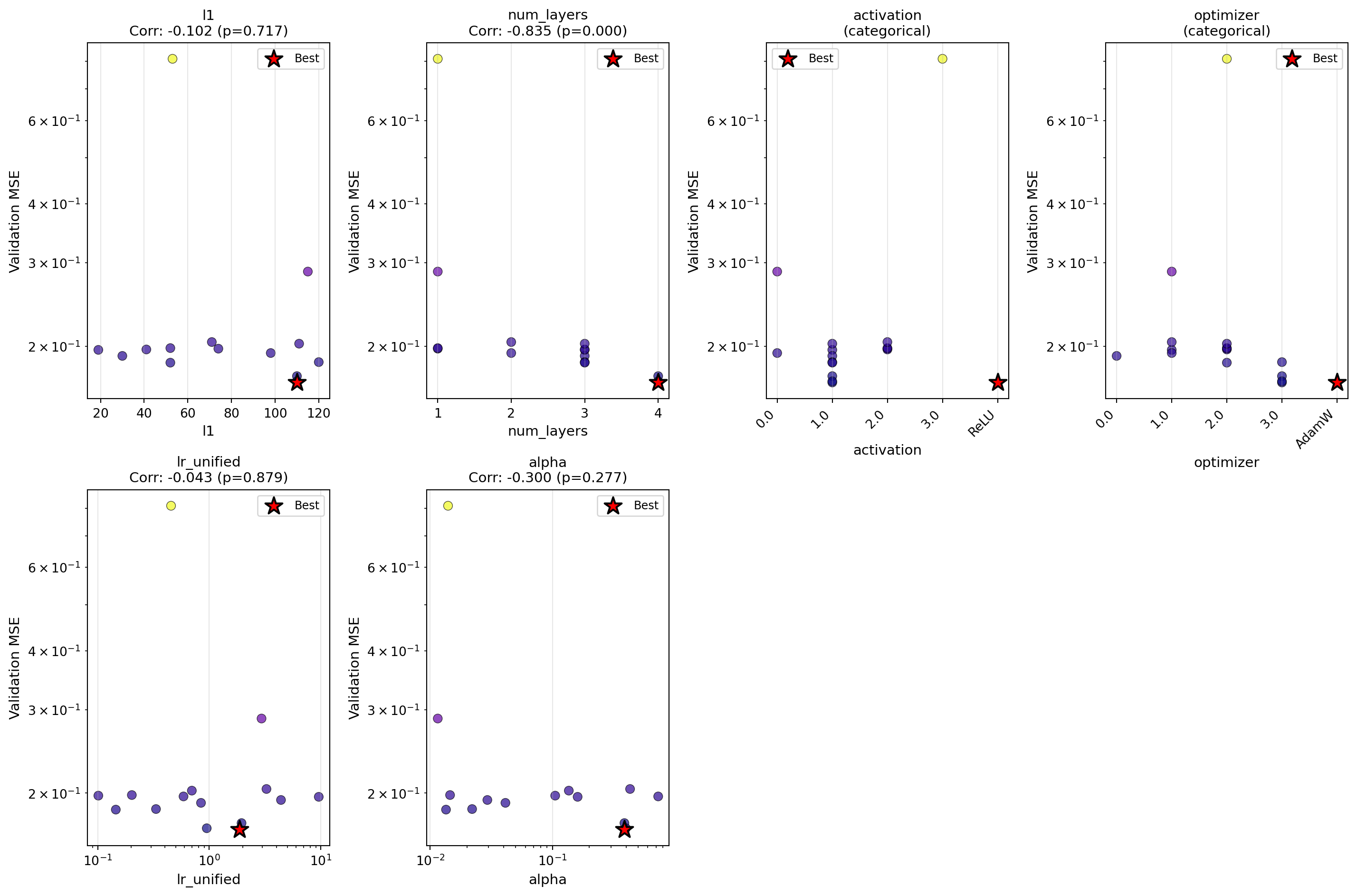
40.1 Sensitivity Analysis (Spearman Correlation)
# Use the new sensitivity_spearman() method for tabular output
optimizer.sensitivity_spearman()
Sensitivity Analysis (Spearman Correlation):
--------------------------------------------------
  l1                  : +0.196 (p=0.483)
  num_layers          : -0.158 (p=0.573)
  activation          : (categorical variable, use visual inspection)
  optimizer           : (categorical variable, use visual inspection)
  lr_unified          : +0.118 (p=0.676)
  alpha               : -0.150 (p=0.594)
41 Summary
41.1 Key Findings
# Get optimization history for statistics
history = optimizer.y_

print("\n" + "="*70)
print("HYPERPARAMETER OPTIMIZATION SUMMARY")
print("="*70)

print("\n1. BEST CONFIGURATION FOUND:")
print(f"   - Neurons per layer (l1): {best_l1}")
print(f"   - Number of hidden layers: {best_num_layers}")
print(f"   - Activation function: {best_activation}")
print(f"   - Optimizer: {best_optimizer}")
print(f"   - Learning rate: {best_lr_unified:.4f}")
print(f"   - Physics weight (alpha): {best_alpha:.4f}")

print("\n2. PERFORMANCE:")
print(f"   - Validation MSE: {best_val_error:.6f}")
print(f"   - Full domain MSE: {full_mse:.6f}")
print(f"   - Maximum absolute error: {max_error:.6f}")

print("\n3. OPTIMIZATION STATISTICS:")
print(f"   - Total evaluations: {result.nfev}")
print(f"   - Initial best: {history[0]:.6f}")
print(f"   - Final best: {best_val_error:.6f}")
print(f"   - Improvement: {(1 - best_val_error/history[0])*100:.1f}%")

print("\n4. COMPARISON TO BASELINE:")
print(f"   - Baseline MSE: {baseline_error:.6f}")
print(f"   - Optimized MSE: {best_val_error:.6f}")
print(f"   - Improvement: {(1 - best_val_error/baseline_error)*100:.1f}%")

print("\n" + "="*70)
======================================================================
HYPERPARAMETER OPTIMIZATION SUMMARY
======================================================================

1. BEST CONFIGURATION FOUND:
   - Neurons per layer (l1): 96
   - Number of hidden layers: 3
   - Activation function: GELU
   - Optimizer: RMSprop
   - Learning rate: 0.2996
   - Physics weight (alpha): 0.1593

2. PERFORMANCE:
   - Validation MSE: 0.169332
   - Full domain MSE: 0.002078
   - Maximum absolute error: 0.119569

3. OPTIMIZATION STATISTICS:
   - Total evaluations: 15
   - Initial best: 0.192541
   - Final best: 0.169332
   - Improvement: 12.1%

4. COMPARISON TO BASELINE:
   - Baseline MSE: 0.185787
   - Optimized MSE: 0.169332
   - Improvement: 8.9%

======================================================================
41.2 Recommendations
Based on the hyperparameter optimization results:
Network Architecture:
- The optimal architecture was found with
{best_l1}neurons and{best_num_layers}hidden layers - Best activation function:
{best_activation} - This balances model capacity with training efficiency
- The optimal architecture was found with
Optimizer Selection:
- Best optimizer:
{best_optimizer} - Different optimizers have different convergence characteristics for PINNs
- Best optimizer:
Learning Rate:
- Optimal unified learning rate:
{best_lr_unified:.4f} - This translates to an actual Adam learning rate of
{best_lr_unified * 0.001:.6f}
- Optimal unified learning rate:
Physics Loss Weight:
- Optimal alpha:
{best_alpha:.4f} - This balances data fitting with physics constraint satisfaction
- Optimal alpha:
Training Strategy:
- Start with a broad search space to explore different architectures
- Use
var_transwith “log10” for learning rate and physics weight parameters - This enables efficient exploration of log-scale parameters without manual transformations
- Validate on held-out data to prevent overfitting to training points
Benefits of var_trans and Factor Variables:
- Factor variables: Categorical choices (activation, optimizer) handled automatically
- SpotOptim maps strings to integers internally and back to strings in results
- Cleaner code: No manual
10**xconversions in objective function - Fewer errors: Eliminates confusion about which scale values are in
- Better optimization: Searches efficiently in transformed space
- Easier interpretation: All results displayed in original scale
41.3 Using These Results
To use the optimized configuration in your own PINN problems:
# Create optimized PINN
model = LinearRegressor(
    input_dim=1,
    output_dim=1,
    l1={best_l1},
    num_hidden_layers={best_num_layers},
    activation="{best_activation}",
    lr={best_lr_unified:.4f}
)

optimizer = model.get_optimizer("{best_optimizer}")

# Use alpha={best_alpha:.4f} for physics loss weight
loss = data_loss + {best_alpha:.4f} * physics_loss
41.4 Using var_trans for Your Hyperparameter Optimization
When setting up optimization for your own PINN problems:
from spotoptim import SpotOptim

# Define search space with factor variables and log-scale parameters
bounds = [
    (16, 128),                                    # neurons (integer)
    (1, 4),                                       # layers (integer)
    ("Tanh", "ReLU", "Sigmoid", "GELU"),       # activation (factor)
    ("Adam", "SGD", "RMSprop", "AdamW"),        # optimizer (factor)
    (0.1, 10.0),                                  # learning rate (log-scale)
    (0.01, 1.0)                                   # physics weight (log-scale)
]

var_type = ["int", "int", "factor", "factor", "float", "float"]
var_trans = [None, None, None, None, "log10", "log10"]

opt = SpotOptim(
    fun=your_objective_function,
    bounds=bounds,
    var_type=var_type,
    var_trans=var_trans,  # Automatic log-scale and factor handling!
    max_iter=MAX_ITER,
    n_initial=N_INITIAL
)

result = opt.optimize()
Your objective function receives parameters in original scale - no manual transformations needed!
41.5 Future Directions
Consider exploring:
- Adaptive physics weights that change during training
- Architecture search including skip connections or residual blocks
- Batch size optimization as an additional hyperparameter
- Multi-objective optimization balancing accuracy and computational cost
- Transfer learning from pre-optimized configurations
- Learning rate schedules with different decay strategies
Note: The specific optimal values depend on the problem, data distribution, and computational budget. Always validate results on held-out test data.
41.6 Jupyter Notebook
Note
- The Jupyter-Notebook of this chapter is available on GitHub in the Sequential Parameter Optimization Cookbook Repository