16  Kriging Surrogate Models in SpotOptim

16.1 Introduction

SpotOptim provides a powerful Kriging (Gaussian Process) surrogate model that can significantly enhance optimization performance. This tutorial introduces the Kriging class, explains its theory and parameters, and demonstrates how to use it effectively with SpotOptim.

16.1.1 What is Kriging?

Kriging, also known as Gaussian Process regression, is a sophisticated interpolation method that:

• Predicts function values at untested points based on observed data
• Provides uncertainty estimates indicating confidence in predictions
• Models smooth functions common in engineering and scientific optimization
• Handles noisy observations through regression approaches

The mathematical foundation of Kriging is based on the assumption that the objective function \(f(\mathbf{x})\) can be modeled as:

\[ f(\mathbf{x}) = \mu + Z(\mathbf{x}) \]

where \(\mu\) is a constant mean and \(Z(\mathbf{x})\) is a Gaussian process with correlation structure. The correlation between two points \(\mathbf{x}_i\) and \(\mathbf{x}_j\) is typically modeled using a Gaussian (RBF) correlation function:

\[ R(\mathbf{x}_i, \mathbf{x}_j) = \exp\left(-\sum_{k=1}^{d} \theta_k |x_{i,k} - x_{j,k}|^2\right) \]

where \(\theta_k > 0\) are the correlation length parameters that control smoothness in each dimension.

16.1.2 Why Use Kriging in SpotOptim?

1. Better Surrogate Models: More accurate predictions than simple interpolation
2. Uncertainty Quantification: Know where the model is uncertain
3. Mixed Variable Types: Handle continuous, integer, and categorical variables
4. Multiple Methods: Choose between interpolation, regression, and reinterpolation
5. Customizable: Control regularization, correlation parameters, and more

16.2 Basic Usage

16.2.1 Creating a Simple Kriging Model

Let’s start with the most basic usage - creating a Kriging model with default settings:

import numpy as np
from spotoptim import SpotOptim
from spotoptim.surrogate import Kriging

# Simple objective function
def sphere(X):
    """Sphere function: f(x) = sum(x^2)"""
    return np.sum(X**2, axis=1)

# Create Kriging surrogate with defaults
kriging = Kriging(seed=42)

# Use with SpotOptim
optimizer = SpotOptim(
    fun=sphere,
    bounds=[(-5, 5), (-5, 5)],
    surrogate=kriging,  # Use Kriging instead of default GP
    max_iter=20,
    n_initial=10,
    seed=42,
    verbose=True
)

result = optimizer.optimize()
print(f"\nBest solution: {result.x}")
print(f"Best value: {result.fun:.6f}")

TensorBoard logging disabled
Initial best: f(x) = 2.420807
Iteration 1: New best f(x) = 0.001740
Iteration 2: New best f(x) = 0.000372
Iteration 3: New best f(x) = 0.000254
Iteration 4: f(x) = 0.004013
Iteration 5: f(x) = 0.001046
Iteration 6: f(x) = 0.001192
Iteration 7: f(x) = 0.001219
Iteration 8: f(x) = 0.001147
Iteration 9: New best f(x) = 0.000004
Iteration 10: New best f(x) = 0.000000

Best solution: [2.04416182e-05 5.67177247e-04]
Best value: 0.000000

16.2.2 Default vs Custom Surrogate

SpotOptim uses a Gaussian Process Regressor by default. Here’s how Kriging compares:

import numpy as np
from spotoptim import SpotOptim
from spotoptim.surrogate import Kriging

def rosenbrock(X):
    """Rosenbrock function: (1-x)^2 + 100(y-x^2)^2"""
    x = X[:, 0]
    y = X[:, 1]
    return (1 - x)**2 + 100 * (y - x**2)**2

# With default Gaussian Process
opt_default = SpotOptim(
    fun=rosenbrock,
    bounds=[(-2, 2), (-2, 2)],
    max_iter=30,
    n_initial=15,
    seed=42,
    verbose=False
)
result_default = opt_default.optimize()

# With Kriging surrogate
kriging = Kriging(method='regression', seed=42)
opt_kriging = SpotOptim(
    fun=rosenbrock,
    bounds=[(-2, 2), (-2, 2)],
    surrogate=kriging,
    max_iter=30,
    n_initial=15,
    seed=42,
    verbose=False
)
result_kriging = opt_kriging.optimize()

print("Comparison:")
print(f"Default GP:  f(x) = {result_default.fun:.6f}")
print(f"Kriging:     f(x) = {result_kriging.fun:.6f}")

Comparison:
Default GP:  f(x) = 0.190180
Kriging:     f(x) = 0.001073

Both approaches work well, but Kriging offers more control over the surrogate behavior.

16.3 Understanding Kriging Parameters

16.3.1 Method: Interpolation vs Regression

The method parameter controls how Kriging handles data:

• “interpolation”: Exact interpolation, passes through all training points
• “regression”: Allows smoothing, better for noisy data
• “reinterpolation”: Hybrid approach

import numpy as np
from spotoptim.surrogate import Kriging
import matplotlib.pyplot as plt

# Create noisy training data
np.random.seed(42)
X_train = np.linspace(0, 2*np.pi, 10).reshape(-1, 1)
y_train = np.sin(X_train.ravel()) + 0.1 * np.random.randn(10)

# Test data for smooth predictions
X_test = np.linspace(0, 2*np.pi, 100).reshape(-1, 1)
y_true = np.sin(X_test.ravel())

# Compare methods
methods = ['interpolation', 'regression', 'reinterpolation']
fig, axes = plt.subplots(1, 3, figsize=(15, 4))

for ax, method in zip(axes, methods):
    model = Kriging(method=method, seed=42, model_fun_evals=50)
    model.fit(X_train, y_train)
    y_pred, y_std = model.predict(X_test, return_std=True)
    
    # Plot
    ax.plot(X_test, y_true, 'k--', label='True function', linewidth=2)
    ax.plot(X_test, y_pred, 'b-', label='Prediction', linewidth=2)
    ax.fill_between(X_test.ravel(), 
                     y_pred - 2*y_std, 
                     y_pred + 2*y_std, 
                     alpha=0.3, label='95% CI')
    ax.scatter(X_train, y_train, c='r', s=50, zorder=5, label='Training data')
    ax.set_title(f'Method: {method}')
    ax.set_xlabel('x')
    ax.set_ylabel('y')
    ax.legend()
    ax.grid(True, alpha=0.3)

plt.tight_layout()
plt.show()

print("Key differences:")
print("- Interpolation: Passes exactly through training points")
print("- Regression: Smooths over noisy data (recommended)")
print("- Reinterpolation: Balances between the two")

Key differences:
- Interpolation: Passes exactly through training points
- Regression: Smooths over noisy data (recommended)
- Reinterpolation: Balances between the two

Recommendation: Use method='regression' for most optimization problems, especially with noisy objectives.

16.3.2 Noise Parameter and Regularization

The noise parameter adds a small nugget effect for numerical stability:

import numpy as np
from spotoptim import SpotOptim
from spotoptim.surrogate import Kriging

def noisy_ackley(X):
    """Ackley function with observation noise"""
    a = 20
    b = 0.2
    c = 2 * np.pi
    n = X.shape[1]
    
    sum_sq = np.sum(X**2, axis=1)
    sum_cos = np.sum(np.cos(c * X), axis=1)
    
    base = -a * np.exp(-b * np.sqrt(sum_sq / n)) - np.exp(sum_cos / n) + a + np.e
    noise = np.random.normal(0, 0.5, size=base.shape)  # Add noise
    return base + noise

# Very small noise (near interpolation)
kriging_small = Kriging(noise=1e-10, method='interpolation', seed=42)
opt_small = SpotOptim(
    fun=noisy_ackley,
    bounds=[(-5, 5), (-5, 5)],
    surrogate=kriging_small,
    max_iter=25,
    n_initial=12,
    seed=42,
    verbose=False
)
result_small = opt_small.optimize()

# Larger noise (more robust to noise)
kriging_large = Kriging(noise=0.01, method='interpolation', seed=42)
opt_large = SpotOptim(
    fun=noisy_ackley,
    bounds=[(-5, 5), (-5, 5)],
    surrogate=kriging_large,
    max_iter=25,
    n_initial=12,
    seed=42,
    verbose=False
)
result_large = opt_large.optimize()

print("Impact of noise parameter:")
print(f"Small noise (1e-10): f(x) = {result_small.fun:.6f}")
print(f"Large noise (0.01):  f(x) = {result_large.fun:.6f}")
print("\nNote: For noisy functions, use 'regression' method instead,")
print("      which automatically optimizes the Lambda (nugget) parameter.")

Impact of noise parameter:
Small noise (1e-10): f(x) = 0.049827
Large noise (0.01):  f(x) = 0.012636

Note: For noisy functions, use 'regression' method instead,
      which automatically optimizes the Lambda (nugget) parameter.

Best Practice: For noisy functions, use method='regression' which automatically optimizes the regularization parameter instead of fixing it.

16.3.3 Correlation Length Parameters (Theta)

The theta parameters control smoothness. SpotOptim optimizes these automatically:

• min_theta: Minimum log₁₀(θ) value (default: -3.0 → θ = 0.001)
• max_theta: Maximum log₁₀(θ) value (default: 2.0 → θ = 100)

Smaller θ → smoother function, larger θ → more wiggly function.

import numpy as np
from spotoptim.surrogate import Kriging

# Sample data
X_train = np.array([[0.0], [0.5], [1.0], [1.5], [2.0]])
y_train = np.sin(X_train.ravel())

# Tight bounds (smoother)
model_smooth = Kriging(min_theta=-1.0, max_theta=0.0, seed=42, model_fun_evals=30)
model_smooth.fit(X_train, y_train)

# Wide bounds (more flexible)
model_flexible = Kriging(min_theta=-3.0, max_theta=2.0, seed=42, model_fun_evals=30)
model_flexible.fit(X_train, y_train)

print("Theta bounds and optimal values:")
print(f"Smooth model:   bounds=[-1.0, 0.0], theta={model_smooth.theta_}")
print(f"Flexible model: bounds=[-3.0, 2.0], theta={model_flexible.theta_}")
print("\nThe optimizer automatically finds the best theta within the bounds.")

Theta bounds and optimal values:
Smooth model:   bounds=[-1.0, 0.0], theta=[-0.95216449]
Flexible model: bounds=[-3.0, 2.0], theta=[-0.95309049]

The optimizer automatically finds the best theta within the bounds.

Default Values: The defaults min_theta=-3.0 and max_theta=2.0 work well for most problems.

16.3.4 Isotropic vs Anisotropic Correlation

• Isotropic (isotropic=True): Single θ for all dimensions (faster, fewer parameters)
• Anisotropic (isotropic=False): Different θ per dimension (more flexible, default)

import numpy as np
from spotoptim.surrogate import Kriging

# 3D problem
np.random.seed(42)
X_train = np.random.rand(15, 3) * 10 - 5
y_train = X_train[:, 0]**2 + 0.1*X_train[:, 1]**2 + 2*X_train[:, 2]**2

# Isotropic: one theta for all dimensions
model_iso = Kriging(isotropic=True, seed=42, model_fun_evals=40)
model_iso.fit(X_train, y_train)

# Anisotropic: different theta per dimension
model_aniso = Kriging(isotropic=False, seed=42, model_fun_evals=40)
model_aniso.fit(X_train, y_train)

print("Correlation structure:")
print(f"Isotropic:   n_theta={model_iso.n_theta}, theta={model_iso.theta_}")
print(f"Anisotropic: n_theta={model_aniso.n_theta}, theta={model_aniso.theta_}")
print("\nAnisotropic can capture different smoothness in each dimension.")

# Test predictions
X_test = np.array([[0.0, 0.0, 0.0]])
y_iso = model_iso.predict(X_test)
y_aniso = model_aniso.predict(X_test)
print(f"\nPrediction at origin:")
print(f"Isotropic:   {y_iso[0]:.4f}")
print(f"Anisotropic: {y_aniso[0]:.4f}")

Correlation structure:
Isotropic:   n_theta=1, theta=[-3.]
Anisotropic: n_theta=3, theta=[-2.23292358 -3.         -1.97228776]

Anisotropic can capture different smoothness in each dimension.

Prediction at origin:
Isotropic:   -0.0666
Anisotropic: -1.0267

When to Use:

• Use isotropic for faster fitting when dimensions have similar characteristics
• Use anisotropic (default) when dimensions behave differently

16.4 Advanced Features

16.4.1 Mixed Variable Types

Kriging supports mixed variable types: continuous (float), integer (int), and categorical (factor):

import numpy as np
from spotoptim import SpotOptim
from spotoptim.surrogate import Kriging

def mixed_objective(X):
    """
    Optimize a system with:
    - x0: continuous learning rate (0.001 to 0.1)
    - x1: integer number of layers (1 to 5)
    - x2: categorical activation (0=ReLU, 1=Tanh, 2=Sigmoid)
    """
    X = np.atleast_2d(X)
    learning_rate = X[:, 0]
    n_layers = X[:, 1]
    activation = X[:, 2]
    
    # Simplified model: prefer lr~0.01, 3 layers, ReLU
    loss = (learning_rate - 0.01)**2 + (n_layers - 3)**2
    loss += np.where(activation == 0, 0.0,  # ReLU is best
                     np.where(activation == 1, 0.5,  # Tanh is ok
                              1.0))  # Sigmoid is worst
    return loss

# Define bounds and types
bounds = [
    (0.001, 0.1),  # learning_rate (float)
    (1, 5),        # n_layers (int)
    (0, 2)         # activation (factor: 0, 1, or 2)
]

var_type = ['float', 'int', 'factor']

# Create Kriging with mixed types
kriging_mixed = Kriging(
    method='regression',
    var_type=var_type,
    seed=42,
    model_fun_evals=50
)

# Optimize
optimizer = SpotOptim(
    fun=mixed_objective,
    bounds=bounds,
    var_type=var_type,
    surrogate=kriging_mixed,
    max_iter=30,
    n_initial=15,
    seed=42,
    verbose=True
)

result = optimizer.optimize()

print(f"\nOptimal configuration:")
print(f"Learning rate: {result.x[0]:.4f}")
print(f"Num layers:    {int(result.x[1])}")
print(f"Activation:    {int(result.x[2])} (0=ReLU, 1=Tanh, 2=Sigmoid)")
print(f"Loss:          {result.fun:.6f}")

TensorBoard logging disabled
Initial best: f(x) = 0.000173
Iteration 1: New best f(x) = 0.000081
  Attempt 2/10: Previous point was duplicate after rounding, trying fallback
Acquisition failure: Using random space-filling design as fallback.
Iteration 2: f(x) = 1.507094
  Attempt 2/10: Previous point was duplicate after rounding, trying fallback
Acquisition failure: Using random space-filling design as fallback.
Iteration 3: f(x) = 0.000599
  Attempt 2/10: Previous point was duplicate after rounding, trying fallback
Acquisition failure: Using random space-filling design as fallback.
Iteration 4: f(x) = 0.000587
  Attempt 2/10: Previous point was duplicate after rounding, trying fallback
Acquisition failure: Using random space-filling design as fallback.
Iteration 5: f(x) = 5.005398
  Attempt 2/10: Previous point was duplicate after rounding, trying fallback
Acquisition failure: Using random space-filling design as fallback.
Iteration 6: f(x) = 1.000342
  Attempt 2/10: Previous point was duplicate after rounding, trying fallback
Acquisition failure: Using random space-filling design as fallback.
Iteration 7: f(x) = 1.501632
  Attempt 2/10: Previous point was duplicate after rounding, trying fallback
Acquisition failure: Using random space-filling design as fallback.
Iteration 8: f(x) = 0.502100
  Attempt 2/10: Previous point was duplicate after rounding, trying fallback
Acquisition failure: Using random space-filling design as fallback.
Iteration 9: f(x) = 2.000762
  Attempt 2/10: Previous point was duplicate after rounding, trying fallback
Acquisition failure: Using random space-filling design as fallback.
Iteration 10: f(x) = 4.006134
  Attempt 2/10: Previous point was duplicate after rounding, trying fallback
Acquisition failure: Using random space-filling design as fallback.
Iteration 11: f(x) = 1.000430
  Attempt 2/10: Previous point was duplicate after rounding, trying fallback
Acquisition failure: Using random space-filling design as fallback.
Iteration 12: f(x) = 1.500167
Iteration 13: New best f(x) = 0.000030
Iteration 14: f(x) = 0.000049
Iteration 15: New best f(x) = 0.000003

Optimal configuration:
Learning rate: 0.0082
Num layers:    3
Activation:    0 (0=ReLU, 1=Tanh, 2=Sigmoid)
Loss:          0.000003

Key Points:

• Set var_type in both Kriging and SpotOptim
• Factor variables use specialized distance metrics (default: Canberra)
• Integer variables are treated as ordered but discrete

16.4.2 Customizing the Distance Metric for Factors

For categorical variables, you can choose different distance metrics.

import numpy as np
from spotoptim.surrogate import Kriging

# Categorical data: 2 factor variables
X_train = np.array([
    [0, 0],  # Category A, Color Red
    [1, 0],  # Category B, Color Red
    [0, 1],  # Category A, Color Blue
    [1, 1],  # Category B, Color Blue
    [2, 2],  # Category C, Color Green
])
y_train = np.array([1.0, 1.5, 1.2, 2.0, 3.5])

# Different distance metrics
metrics = ['canberra', 'hamming']

for metric in metrics:
    model = Kriging(
        method='regression',
        var_type=['factor', 'factor'],
        metric_factorial=metric,
        seed=42,
        model_fun_evals=40
    )
    model.fit(X_train, y_train)
    
    # Test prediction
    X_test = np.array([[1, 1]])
    y_pred = model.predict(X_test)
    
    print(f"Metric: {metric:10s} | Prediction at [1,1]: {y_pred[0]:.4f}")

print("\nAvailable metrics: 'canberra' (default), 'hamming', 'jaccard', etc.")

Metric: canberra   | Prediction at [1,1]: 1.9463
Metric: hamming    | Prediction at [1,1]: 2.0000

Available metrics: 'canberra' (default), 'hamming', 'jaccard', etc.

16.4.3 Handling High-Dimensional Problems

For high-dimensional problems, Kriging can become computationally expensive. Here are strategies:

import numpy as np
from spotoptim import SpotOptim
from spotoptim.surrogate import Kriging

def high_dim_sphere(X):
    """10-dimensional sphere function"""
    return np.sum(X**2, axis=1)

# Strategy 1: Use isotropic correlation (fewer parameters)
kriging_iso = Kriging(
    method='regression',
    isotropic=True,  # Single theta for all 10 dimensions
    seed=42,
    model_fun_evals=50  # Faster optimization
)

optimizer_iso = SpotOptim(
    fun=high_dim_sphere,
    bounds=[(-5, 5)] * 10,  # 10 dimensions
    surrogate=kriging_iso,
    max_iter=50,
    n_initial=30,
    seed=42,
    verbose=False
)

result_iso = optimizer_iso.optimize()

# Strategy 2: Use max_surrogate_points to limit training set size
kriging_limited = Kriging(method='regression', seed=42)

optimizer_limited = SpotOptim(
    fun=high_dim_sphere,
    bounds=[(-5, 5)] * 10,
    surrogate=kriging_limited,
    max_iter=50,
    n_initial=30,
    max_surrogate_points=100,  # Limit surrogate training set
    seed=42,
    verbose=False
)

result_limited = optimizer_limited.optimize()

print("High-dimensional optimization strategies:")
print(f"Isotropic Kriging:      f(x) = {result_iso.fun:.6f}")
print(f"Limited training set:   f(x) = {result_limited.fun:.6f}")
print("\nFor >5 dimensions, consider isotropic=True or limit training set.")

High-dimensional optimization strategies:
Isotropic Kriging:      f(x) = 0.003979
Limited training set:   f(x) = 0.044950

For >5 dimensions, consider isotropic=True or limit training set.

16.4.4 Uncertainty Quantification

Kriging provides uncertainty estimates, useful for exploration vs exploitation:

import numpy as np
from spotoptim.surrogate import Kriging
import matplotlib.pyplot as plt

# 1D example for visualization
np.random.seed(42)
X_train = np.array([[0.0], [1.0], [3.0], [5.0], [6.0]])
y_train = np.sin(X_train.ravel()) + 0.05 * np.random.randn(5)

# Fit Kriging model
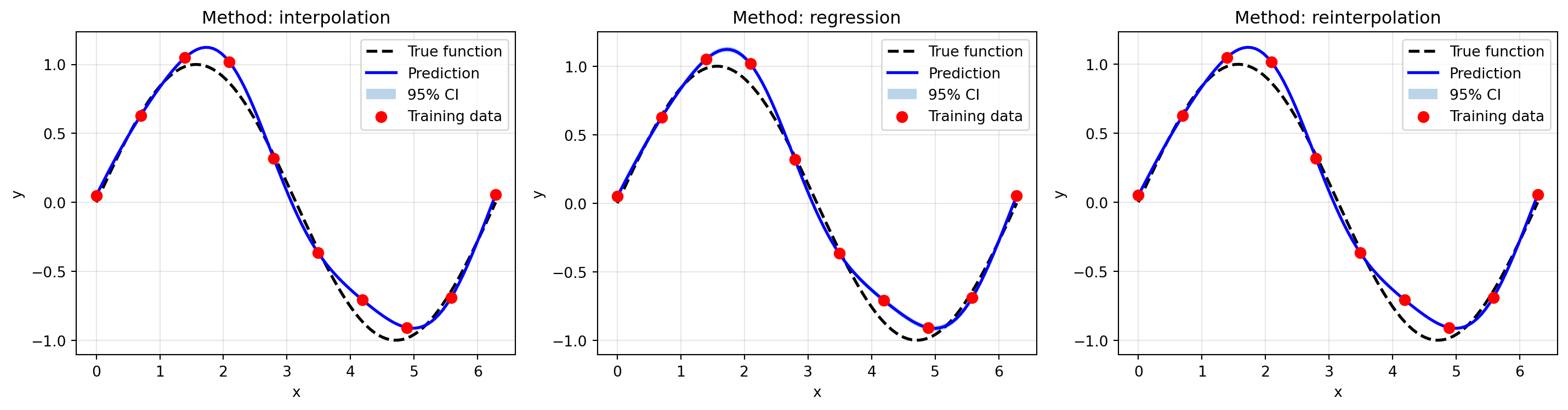
model = Kriging(method='regression', seed=42, model_fun_evals=50)
model.fit(X_train, y_train)

# Dense test points
X_test = np.linspace(-0.5, 6.5, 200).reshape(-1, 1)
y_pred, y_std = model.predict(X_test, return_std=True)

# True function
y_true = np.sin(X_test.ravel())

# Plot
plt.figure(figsize=(12, 5))

plt.subplot(1, 2, 1)
plt.plot(X_test, y_true, 'k--', label='True function', linewidth=2)
plt.plot(X_test, y_pred, 'b-', label='Kriging prediction', linewidth=2)
plt.fill_between(X_test.ravel(), 
                 y_pred - 2*y_std, 
                 y_pred + 2*y_std, 
                 alpha=0.3, color='blue', label='95% confidence')
plt.scatter(X_train, y_train, c='red', s=100, zorder=5, 
           edgecolors='black', label='Training points')
plt.xlabel('x', fontsize=12)
plt.ylabel('y', fontsize=12)
plt.title('Kriging Predictions with Uncertainty', fontsize=14)
plt.legend()
plt.grid(True, alpha=0.3)

plt.subplot(1, 2, 2)
plt.plot(X_test, y_std, 'r-', linewidth=2)
plt.scatter(X_train, np.zeros_like(X_train), c='blue', s=100, 
           zorder=5, edgecolors='black', label='Training points')
plt.xlabel('x', fontsize=12)
plt.ylabel('Standard Deviation', fontsize=12)
plt.title('Uncertainty Estimates', fontsize=14)
plt.legend()
plt.grid(True, alpha=0.3)

plt.tight_layout()
plt.show()

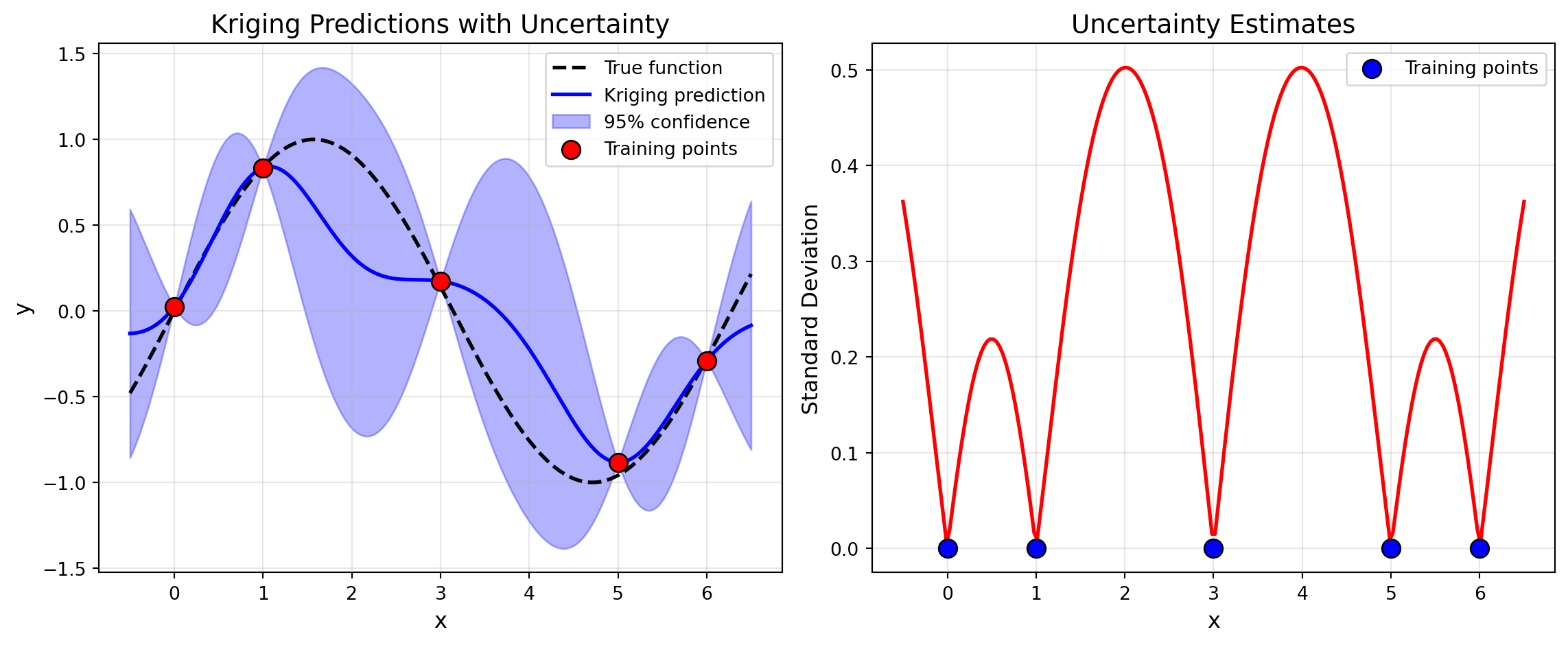
print("Key observations:")
print("- Uncertainty is low near training points")
print("- Uncertainty is high far from training data")
print("- This guides acquisition functions (e.g., EI exploits low uncertainty)")

Key observations:
- Uncertainty is low near training points
- Uncertainty is high far from training data
- This guides acquisition functions (e.g., EI exploits low uncertainty)

16.5 Practical Examples

16.5.1 Example 1: Optimizing the Rastrigin Function

The Rastrigin function is highly multimodal - a challenging test case:

import numpy as np
from spotoptim import SpotOptim
from spotoptim.surrogate import Kriging

def rastrigin(X):
    """
    Rastrigin function: highly multimodal
    Global minimum: f(0,...,0) = 0
    """
    A = 10
    n = X.shape[1]
    return A * n + np.sum(X**2 - A * np.cos(2 * np.pi * X), axis=1)

# Configure Kriging for multimodal function
kriging = Kriging(
    method='regression',      # Smooth over local variations
    min_theta=-3.0,          # Allow flexible correlation
    max_theta=2.0,
    seed=42,
    model_fun_evals=100      # More budget for better surrogate
)

optimizer = SpotOptim(
    fun=rastrigin,
    bounds=[(-5.12, 5.12), (-5.12, 5.12)],
    surrogate=kriging,
    acquisition='ei',         # Expected Improvement for exploration
    max_iter=60,
    n_initial=30,
    seed=42,
    verbose=True
)

result = optimizer.optimize()

print(f"\nRastrigin optimization:")
print(f"Best solution: {result.x}")
print(f"Best value:    {result.fun:.6f} (global optimum: 0.0)")
print(f"Distance to optimum: {np.linalg.norm(result.x):.6f}")

TensorBoard logging disabled
Initial best: f(x) = 6.442225
Iteration 1: f(x) = 28.951536
Iteration 2: f(x) = 22.875749
Iteration 3: f(x) = 21.815864
Iteration 4: f(x) = 7.077873
Iteration 5: f(x) = 13.368250
Iteration 6: f(x) = 16.577976
Iteration 7: f(x) = 25.780045
Iteration 8: f(x) = 10.034344
Iteration 9: f(x) = 19.560557
Iteration 10: f(x) = 12.381235
Iteration 11: f(x) = 20.126829
Iteration 12: f(x) = 27.151349
Iteration 13: New best f(x) = 2.290927
Iteration 14: f(x) = 2.761961
Iteration 15: f(x) = 12.468354
Iteration 16: New best f(x) = 1.208377
Iteration 17: f(x) = 12.566211
Iteration 18: f(x) = 14.965620
Iteration 19: f(x) = 14.295554
Iteration 20: f(x) = 28.107905
Iteration 21: f(x) = 22.687907
Iteration 22: f(x) = 43.729592
Iteration 23: f(x) = 41.636148
Iteration 24: New best f(x) = 1.034573
Iteration 25: f(x) = 3.228327
Iteration 26: f(x) = 7.934136
Iteration 27: f(x) = 21.994039
Iteration 28: f(x) = 27.510661
Iteration 29: f(x) = 9.365219
Iteration 30: f(x) = 1.248535

Rastrigin optimization:
Best solution: [-0.00987679  1.00506675]
Best value:    1.034573 (global optimum: 0.0)
Distance to optimum: 1.005115

16.5.2 Example 2: Robust Optimization with Noise

When optimizing noisy functions, Kriging’s regression mode helps:

import numpy as np
from spotoptim import SpotOptim
from spotoptim.surrogate import Kriging

def noisy_beale(X):
    """
    Beale function with Gaussian noise
    Global minimum: f(3, 0.5) = 0
    """
    x = X[:, 0]
    y = X[:, 1]
    
    term1 = (1.5 - x + x * y)**2
    term2 = (2.25 - x + x * y**2)**2
    term3 = (2.625 - x + x * y**3)**2
    
    base = term1 + term2 + term3
    noise = np.random.normal(0, 0.5, size=base.shape)
    
    return base + noise

# Use regression method for noisy objectives
kriging_robust = Kriging(
    method='regression',        # Automatically optimizes Lambda (nugget)
    min_Lambda=-9.0,           # Allow small regularization
    max_Lambda=-2.0,           # But not too large
    seed=42,
    model_fun_evals=80
)

# Use repeated evaluations for noise handling
optimizer = SpotOptim(
    fun=noisy_beale,
    bounds=[(-4.5, 4.5), (-4.5, 4.5)],
    surrogate=kriging_robust,
    max_iter=50,
    n_initial=20,
    repeats_initial=3,         # Evaluate each initial point 3 times
    repeats_surrogate=2,       # Evaluate each new point 2 times
    seed=42,
    verbose=True
)

result = optimizer.optimize()

print(f"\nNoisy Beale optimization:")
print(f"Best solution: {result.x}")
print(f"Best mean value: {optimizer.min_mean_y:.6f}")
print(f"Variance at best: {optimizer.min_var_y:.6f}")
print(f"True optimum: [3.0, 0.5]")
print(f"Distance: {np.linalg.norm(result.x - np.array([3.0, 0.5])):.4f}")

TensorBoard logging disabled
Initial best: f(x) = 9.379814, mean best: f(x) = 9.729582

Noisy Beale optimization:
Best solution: [ 0.34789079 -0.3014163 ]
Best mean value: 9.729582
Variance at best: 0.214586
True optimum: [3.0, 0.5]
Distance: 2.7706

16.5.3 Example 3: Real-World Machine Learning Hyperparameter Tuning

Optimize hyperparameters for a neural network:

import numpy as np
from spotoptim import SpotOptim
from spotoptim.surrogate import Kriging

def ml_objective(X):
    """
    Simulate training a neural network
    Variables:
    - x0: learning_rate (log scale: 1e-4 to 1e-1)
    - x1: num_layers (integer: 1 to 5)
    - x2: hidden_size (integer: 16, 32, 64, 128, 256)
    - x3: dropout_rate (float: 0.0 to 0.5)
    
    Returns validation error
    """
    X = np.atleast_2d(X)
    lr = X[:, 0]
    n_layers = X[:, 1]
    hidden_size = X[:, 2]
    dropout = X[:, 3]
    
    # Simulate validation error (lower is better)
    # Optimal around: lr=0.001, 3 layers, 64 hidden, 0.2 dropout
    error = (np.log10(lr) + 3)**2  # Prefer lr ~ 0.001
    error += (n_layers - 3)**2     # Prefer 3 layers
    error += ((hidden_size - 64) / 32)**2  # Prefer 64 hidden units
    error += (dropout - 0.2)**2 * 10  # Prefer 0.2 dropout
    
    # Add some noise to simulate training variance
    error += np.random.normal(0, 0.1, size=error.shape)
    
    return error

# Setup optimization
bounds = [
    (1e-4, 1e-1),  # learning_rate
    (1, 5),        # num_layers
    (16, 256),     # hidden_size
    (0.0, 0.5)     # dropout_rate
]

var_type = ['float', 'int', 'int', 'float']

# Use Kriging with mixed types
kriging_ml = Kriging(
    method='regression',
    var_type=var_type,
    seed=42,
    model_fun_evals=60
)

optimizer = SpotOptim(
    fun=ml_objective,
    bounds=bounds,
    var_type=var_type,
    var_trans=['log10', None, None, None],  # Log scale for learning rate
    surrogate=kriging_ml,
    max_iter=40,
    n_initial=20,
    seed=42,
    verbose=True
)

result = optimizer.optimize()

print(f"\nOptimal hyperparameters:")
print(f"Learning rate: {result.x[0]:.6f}")
print(f"Num layers:    {int(result.x[1])}")
print(f"Hidden size:   {int(result.x[2])}")
print(f"Dropout rate:  {result.x[3]:.3f}")
print(f"Validation error: {result.fun:.6f}")

TensorBoard logging disabled
Initial best: f(x) = 1.133527
Iteration 1: f(x) = 5.122533
Iteration 2: f(x) = 5.959913
Iteration 3: f(x) = 1.505793
Iteration 4: New best f(x) = 0.942988
Iteration 5: New best f(x) = 0.280219
Iteration 6: New best f(x) = 0.260858
Iteration 7: f(x) = 1.115300
Iteration 8: f(x) = 0.653129
Iteration 9: New best f(x) = 0.176351
Iteration 10: New best f(x) = 0.084523
Iteration 11: New best f(x) = -0.067705
Iteration 12: f(x) = 0.167623
Iteration 13: f(x) = 0.048797
Iteration 14: f(x) = 0.053888
Iteration 15: f(x) = 0.015810
Iteration 16: New best f(x) = -0.108042
Iteration 17: f(x) = -0.007253
Iteration 18: f(x) = -0.003508
Iteration 19: f(x) = -0.052430
Iteration 20: f(x) = 0.006251

Optimal hyperparameters:
Learning rate: 0.000987
Num layers:    3
Hidden size:   68
Dropout rate:  0.158
Validation error: -0.108042

16.5.4 Example 4: Comparing Kriging Methods

Let’s compare all three Kriging methods on the same problem:

import numpy as np
from spotoptim import SpotOptim
from spotoptim.surrogate import Kriging

def levy(X):
    """
    Levy function N. 13
    Global minimum: f(1, 1) = 0
    """
    x = X[:, 0]
    y = X[:, 1]
    
    w1 = 1 + (x - 1) / 4
    w2 = 1 + (y - 1) / 4
    
    term1 = np.sin(np.pi * w1)**2
    term2 = (w1 - 1)**2 * (1 + 10 * np.sin(np.pi * w1 + 1)**2)
    term3 = (w2 - 1)**2 * (1 + np.sin(2 * np.pi * w2)**2)
    
    return term1 + term2 + term3

methods = ['interpolation', 'regression', 'reinterpolation']
results_methods = []

for method in methods:
    kriging = Kriging(
        method=method,
        seed=42,
        model_fun_evals=60
    )
    
    optimizer = SpotOptim(
        fun=levy,
        bounds=[(-10, 10), (-10, 10)],
        surrogate=kriging,
        max_iter=40,
        n_initial=20,
        seed=42,
        verbose=False
    )
    
    result = optimizer.optimize()
    results_methods.append((method, result.fun, result.x))
    
    print(f"{method:15s} | f(x) = {result.fun:8.6f} | x = {result.x}")

print(f"\nGlobal optimum: f(1, 1) = 0.0")
print("\nAll methods find good solutions, but 'regression' is most robust.")

interpolation   | f(x) = 0.001657 | x = [0.98535016 0.85317084]
regression      | f(x) = 0.027480 | x = [0.8385841 1.068918 ]
reinterpolation | f(x) = 0.027480 | x = [0.8385841 1.068918 ]

Global optimum: f(1, 1) = 0.0

All methods find good solutions, but 'regression' is most robust.

16.5.5 Example 5: Sensitivity to Theta Bounds

Theta bounds control the range of smoothness. Let’s see their impact:

import numpy as np
from spotoptim import SpotOptim
from spotoptim.surrogate import Kriging

def griewank(X):
    """Griewank function"""
    sum_sq = np.sum(X**2 / 4000, axis=1)
    prod_cos = np.prod(np.cos(X / np.sqrt(np.arange(1, X.shape[1] + 1))), axis=1)
    return sum_sq - prod_cos + 1

# Different theta bounds
theta_configs = [
    (-2.0, 1.0, "Tight (smoother)"),
    (-3.0, 2.0, "Default"),
    (-4.0, 3.0, "Wide (more flexible)")
]

for min_theta, max_theta, label in theta_configs:
    kriging = Kriging(
        method='regression',
        min_theta=min_theta,
        max_theta=max_theta,
        seed=42,
        model_fun_evals=50
    )
    
    optimizer = SpotOptim(
        fun=griewank,
        bounds=[(-600, 600), (-600, 600)],
        surrogate=kriging,
        max_iter=35,
        n_initial=18,
        seed=42,
        verbose=False
    )
    
    result = optimizer.optimize()
    print(f"{label:20s} [{min_theta:5.1f}, {max_theta:4.1f}] | f(x) = {result.fun:8.6f}")

print("\nDefault bounds work well for most problems.")

Tight (smoother)     [ -2.0,  1.0] | f(x) = 8.578706
Default              [ -3.0,  2.0] | f(x) = 13.108634
Wide (more flexible) [ -4.0,  3.0] | f(x) = 2.652215

Default bounds work well for most problems.

16.6 Comparing Surrogates

16.6.1 Kriging vs Gaussian Process vs Random Forest

Let’s compare different surrogate models:

import numpy as np
from spotoptim import SpotOptim
from spotoptim.surrogate import Kriging, SimpleKriging
from sklearn.gaussian_process import GaussianProcessRegressor
from sklearn.gaussian_process.kernels import Matern, ConstantKernel
from sklearn.ensemble import RandomForestRegressor

def schwefel(X):
    """Schwefel function"""
    return 418.9829 * X.shape[1] - np.sum(X * np.sin(np.sqrt(np.abs(X))), axis=1)

bounds = [(-500, 500), (-500, 500)]

# 1. Kriging (full-featured)
kriging = Kriging(method='regression', seed=42, model_fun_evals=60)
opt_kriging = SpotOptim(fun=schwefel, bounds=bounds, surrogate=kriging,
                        max_iter=35, n_initial=18, seed=42, verbose=False)
result_kriging = opt_kriging.optimize()

# 2. SimpleKriging (lightweight)
simple_kriging = SimpleKriging(noise=1e-10, seed=42)
opt_simple = SpotOptim(fun=schwefel, bounds=bounds, surrogate=simple_kriging,
                       max_iter=35, n_initial=18, seed=42, verbose=False)
result_simple = opt_simple.optimize()

# 3. Gaussian Process (sklearn default)
kernel = ConstantKernel(1.0) * Matern(length_scale=1.0, nu=2.5)
gp = GaussianProcessRegressor(kernel=kernel, n_restarts_optimizer=10,
                               normalize_y=True, random_state=42)
opt_gp = SpotOptim(fun=schwefel, bounds=bounds, surrogate=gp,
                   max_iter=35, n_initial=18, seed=42, verbose=False)
result_gp = opt_gp.optimize()

# 4. Random Forest
rf = RandomForestRegressor(n_estimators=100, random_state=42)
opt_rf = SpotOptim(fun=schwefel, bounds=bounds, surrogate=rf,
                   max_iter=35, n_initial=18, seed=42, verbose=False)
result_rf = opt_rf.optimize()

print("Surrogate Model Comparison:")
print(f"Kriging (full):     f(x) = {result_kriging.fun:8.2f}")
print(f"SimpleKriging:      f(x) = {result_simple.fun:8.2f}")
print(f"Gaussian Process:   f(x) = {result_gp.fun:8.2f}")
print(f"Random Forest:      f(x) = {result_rf.fun:8.2f}")
print(f"\nGlobal optimum: f(420.9687, 420.9687) = 0.0")
print("\nKriging offers:")
print("- Mixed variable types (continuous, integer, categorical)")
print("- Multiple methods (interpolation, regression, reinterpolation)")
print("- Explicit control over regularization and correlation")

Surrogate Model Comparison:
Kriging (full):     f(x) =   118.47
SimpleKriging:      f(x) =   118.44
Gaussian Process:   f(x) =   118.44
Random Forest:      f(x) =   184.74

Global optimum: f(420.9687, 420.9687) = 0.0

Kriging offers:
- Mixed variable types (continuous, integer, categorical)
- Multiple methods (interpolation, regression, reinterpolation)
- Explicit control over regularization and correlation

16.7 Best Practices

16.7.1 1. Choosing the Right Method

# For smooth, deterministic functions
kriging = Kriging(method='interpolation', noise=1e-10, seed=42)

# For general optimization (RECOMMENDED)
kriging = Kriging(method='regression', seed=42)

# For noisy functions with repeated evaluations
kriging = Kriging(method='regression', seed=42)
# Use with repeats_initial and repeats_surrogate in SpotOptim

16.7.2 2. Setting Model Complexity

# For low-dimensional problems (<5D)
kriging = Kriging(
    method='regression',
    isotropic=False,           # Anisotropic (default)
    model_fun_evals=100,       # More budget for better fit
    seed=42
)

# For high-dimensional problems (>5D)
kriging = Kriging(
    method='regression',
    isotropic=True,            # Fewer parameters
    model_fun_evals=50,        # Faster fitting
    seed=42
)

16.7.3 3. Handling Different Variable Types

# Mixed types example
bounds = [
    (0.0, 10.0),    # continuous
    (1, 10),        # integer
    (0, 3)          # categorical (4 categories)
]

var_type = ['float', 'int', 'factor']

kriging = Kriging(
    method='regression',
    var_type=var_type,
    metric_factorial='canberra',  # For factor variables
    seed=42
)

optimizer = SpotOptim(
    fun=objective,
    bounds=bounds,
    var_type=var_type,
    surrogate=kriging,
    seed=42
)

16.7.4 4. Reproducibility

Always set the seed for reproducible results:

# Both Kriging and SpotOptim should have seeds
kriging = Kriging(method='regression', seed=42)

optimizer = SpotOptim(
    fun=objective,
    bounds=bounds,
    surrogate=kriging,
    seed=42  # Same seed or different seed
)

16.7.5 5. Monitoring Surrogate Quality

Check the negative log-likelihood after fitting:

import numpy as np
from spotoptim.surrogate import Kriging

# Sample data
X = np.random.rand(20, 2) * 10 - 5
y = np.sum(X**2, axis=1)

model = Kriging(method='regression', seed=42)
model.fit(X, y)

print(f"Negative log-likelihood: {model.negLnLike:.4f}")
print(f"Optimized theta: {model.theta_}")
print(f"Optimized Lambda: {model.Lambda_:.4f}")
print(f"Condition number of Psi: {model.cnd_Psi:.2e}")

print("\nLower negLnLike = better fit")
print("Check condition number for numerical stability")

Negative log-likelihood: -15.3998
Optimized theta: [-3. -3.]
Optimized Lambda: -8.9957
Condition number of Psi: 4.03e+13

Lower negLnLike = better fit
Check condition number for numerical stability

16.8 Common Issues and Solutions

16.8.1 Issue 1: Slow Fitting for Large Datasets

Problem: Kriging becomes slow with many training points.

Solution: Limit surrogate training set size:

# Use max_surrogate_points in SpotOptim
optimizer = SpotOptim(
    fun=objective,
    bounds=bounds,
    surrogate=kriging,
    max_surrogate_points=200,  # Limit to 200 points
    selection_method='distant', # or 'best'
    seed=42
)

16.8.2 Issue 2: Poor Predictions for Categorical Variables

Problem: Kriging doesn’t handle factors well.

Solution: Try different distance metrics:

# Try different metrics
for metric in ['canberra', 'hamming', 'jaccard']:
    kriging = Kriging(
        method='regression',
        var_type=['float', 'factor'],
        metric_factorial=metric,
        seed=42
    )
    # Test performance

16.8.3 Issue 3: Numerical Instability

Problem: Correlation matrix is nearly singular.

Solution: Increase regularization:

# For interpolation method
kriging = Kriging(
    method='interpolation',
    noise=1e-6,  # Increase from default 1e-8
    seed=42
)

# Or use regression method (recommended)
kriging = Kriging(
    method='regression',
    min_Lambda=-6.0,  # Don't go too small
    seed=42
)

16.8.4 Issue 4: Overfitting to Noisy Data

Problem: Kriging fits noise instead of underlying function.

Solution: Use regression method with reasonable Lambda bounds:

kriging = Kriging(
    method='regression',
    min_Lambda=-5.0,  # Not too small
    max_Lambda=-1.0,  # Not too large
    seed=42
)

16.9 Summary

16.9.1 Key Takeaways

1. Use method='regression' for most optimization problems
2. Set seed for reproducibility
3. Use var_type for mixed variable types
4. Default parameters work well for most cases
5. Use isotropic=True for high-dimensional problems (>5D)

16.9.2 Quick Reference

from spotoptim import SpotOptim
from spotoptim.surrogate import Kriging

# Recommended configuration for general use
kriging = Kriging(
    method='regression',        # Smooths over noise
    seed=42                     # Reproducibility
)

optimizer = SpotOptim(
    fun=objective,
    bounds=bounds,
    surrogate=kriging,
    max_iter=50,
    n_initial=20,
    seed=42,
    verbose=True
)

result = optimizer.optimize()

16.9.3 Parameter Cheat Sheet

Parameter	Default	When to Change
method	'regression'	Use 'interpolation' for exact fit
noise	sqrt(eps)	Rarely; use method='regression' instead
min_theta	-3.0	Adjust if default range doesn’t work
max_theta	2.0	Adjust if default range doesn’t work
isotropic	False	Set True for >5 dimensions
var_type	['num']	Set for mixed variable types
metric_factorial	'canberra'	Try 'hamming' for factors
model_fun_evals	100	Reduce for faster fitting
seed	124	Always set for reproducibility

16.10 Jupyter Notebook

Note

• The Jupyter-Notebook of this chapter is available on GitHub in the Sequential Parameter Optimization Cookbook Repository