Operational diagnostic plots for energy-load forecasting pipelines.
Ports five matplotlib helpers from the chapter-14 team4 operational script (bart26k-lecture/scripts/team4_4zones_submit.py) into a reusable, stateless API. All functions return a matplotlib.figure.Figure; the caller is responsible for saving and closing it. No plt.show() is called and the backend is never changed here (set matplotlib.use("Agg") before importing pyplot in headless environments).
Map a feature name to its diagnostic family label.
This is the public, importable version of the family_of helper used inside the chapter-14 team4 operational script. The mapping is intentionally coarse — it covers the feature names that ConfigEntsoe and ForecasterRecursive generate and is used exclusively for colour grouping in plot_feature_importance_by_family.
from spotforecast2.plots.diagnostics import feature_familyprint(feature_family("holiday_DE"))print(feature_family("brueckentag_NW"))print(feature_family("poly_hour_2"))print(feature_family("window_mean_72"))print(feature_family("sin_hour"))print(feature_family("lag_1"))print(feature_family("wind_speed_10m"))
holiday
holiday
polynomial
weather_window
cyclical/RBF
lag
weather/other
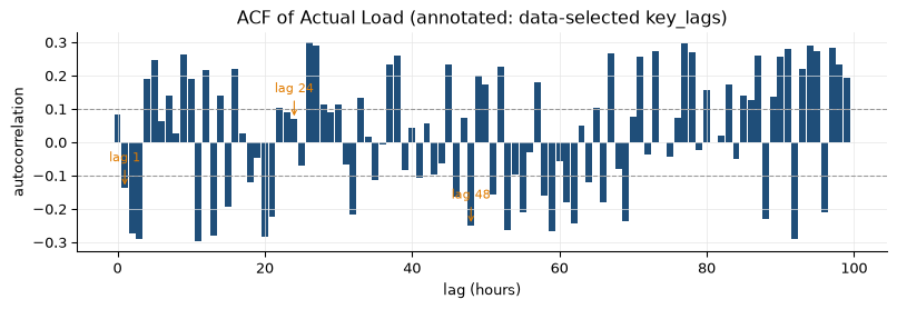
Bar chart of autocorrelation values with annotated key lags.
Ports _plot_acf from the chapter-14 team4 script. The acf DataFrame is the output of spotforecast2.stats.autocorrelation.calculate_lag_autocorrelation and must contain at minimum the columns "lag" and "autocorrelation".
Confidence-band lines at +conf / -conf are drawn as dashed grey horizontal lines. Each lag in key_lags that is present in acf["lag"] gets an orange arrow annotation. Lags not found in the frame are silently skipped.
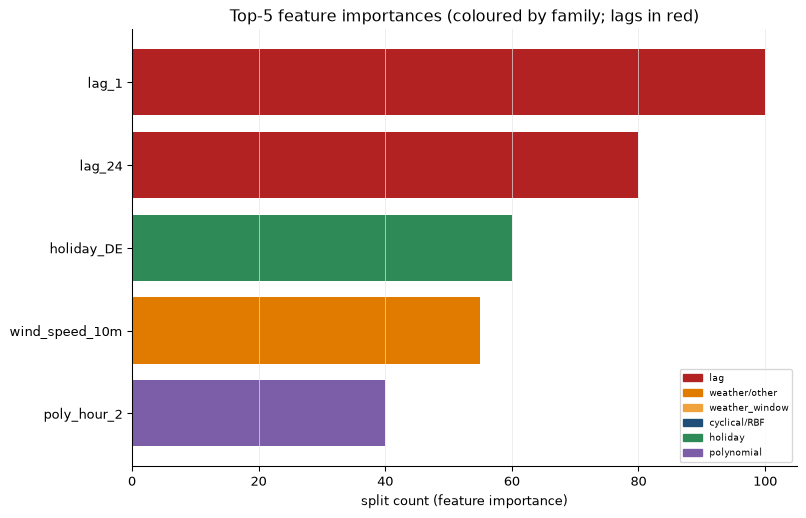
Horizontal bar chart of the top-N feature importances, coloured by family.
Ports _plot_importance from the chapter-14 team4 script. Feature families are determined by feature_family; the colour palette is the same as in the script so diagnostics look identical.
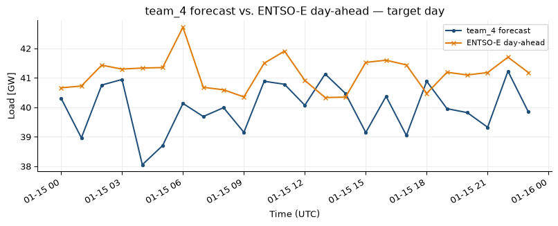
Line plot comparing a forecast against an optional reference series.
Ports _plot_vs_entsoe from the chapter-14 team4 script into a general, label-parametrised form. The reference is reindexed to forecast.index; only the overlapping (non-NaN) timestamps are plotted. If there is no overlap the reference line is omitted and an INFO message is logged — the function still returns a valid single-line figure rather than raising.
Both series are scaled by unit_scale before plotting (default 1e-3 converts MW to GW).
The overlap MAD (mean absolute deviation between forecast and reference over shared timestamps) is logged at INFO level when an overlap exists. This mirrors the original script’s behaviour and is useful for post-hoc sanity checks in operator logs.
Reference series (e.g. ENTSO-E day-ahead forecast). Will be reindexed to forecast.index; NaN rows after reindexing are treated as “no overlap” for that timestamp.
Ports _plot_shap from the chapter-14 team4 script. X is subsampled to approximately max_samples rows (uniform stride len(X) // max_samples; lengths just above max_samples are passed in full) before computing SHAP values so the call stays fast even for large training matrices.
The function uses shap.TreeExplainer and shap.summary_plot(plot_type="bar", show=False), then captures the current matplotlib figure via plt.gcf(). Because the figure is harvested from the global pyplot state this function is not thread-safe. Callers must close the returned figure (e.g. plt.close(fig)) before performing other pyplot work.